You can easily spot and highlight important facts about your data with Excel’s formatting features, including negative numbers.
Losses are usually displayed in red numbers in financial reports, such as company profit and loss statements. Using the same techniques, you can display negative values in any color that is convenient for you. In addition to making them easier to see, this red font color is also convenient.
It can be difficult to locate negative numbers right away when browsing your Excel worksheet if it contains many negative numbers. By custom formatting the selected cells, or conditionally formatting all of them at once, you can actually mark all negative numbers in red. In Excel, you can highlight and mark only certain data in the data set in a variety of ways (such as using conditional formatting, inbuilt number formatting, etc.) to highlight and mark only certain numbers in the current worksheet.
In this gearupwindows article, you will learn how to highlight negative numbers in Excel.
How to Highlight Cells with Negative Values using Conditional Formatting?
If the value in a cell is less than zero (0) that will be a negative number. So, we can highlight it in a specified color (which is red in this example) based on Excel Conditional Formatting rules. Here is how to do it.
Step 1. First, you’ll need to select a range of cells that contain the numbers.
Step 2. Then, click on the Home tab in the menu bar.
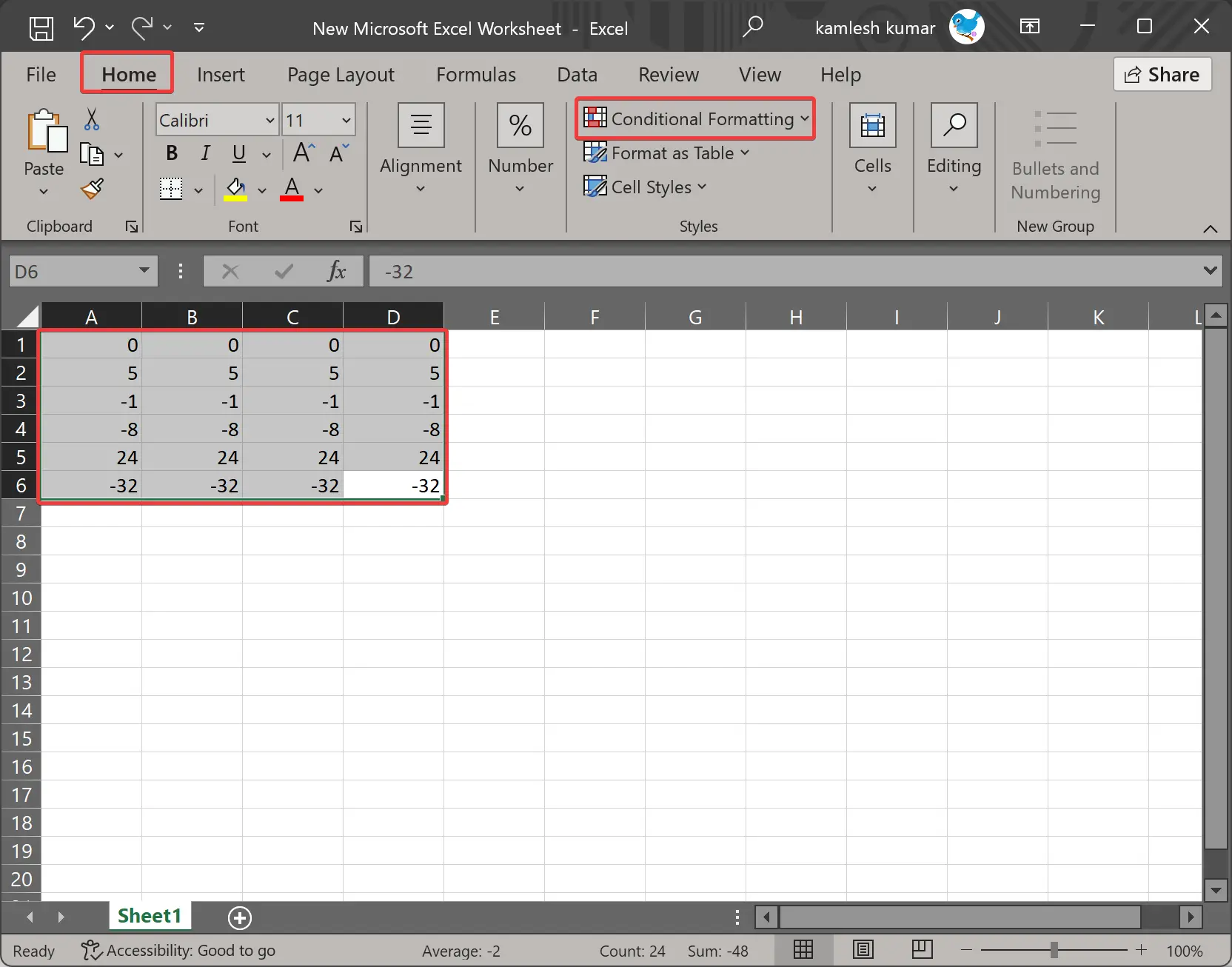
Step 3. In the Styles group, click the Conditional Formatting button.
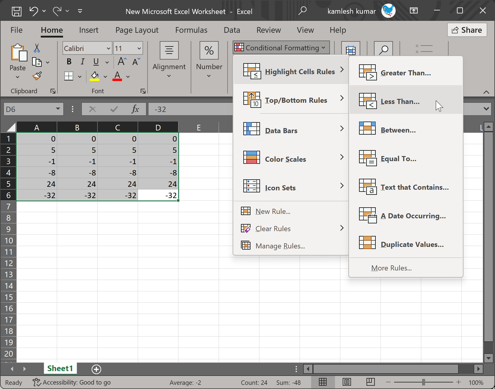
Step 4. Select Highlight Cells Rules > Less Than in the drop-down menu.
Step 5. When you’re done, a “Less Than” dialog box will appear on the screen. Click the drop-down arrow and select a highlight option, for instance, Light red fill with dark red text.
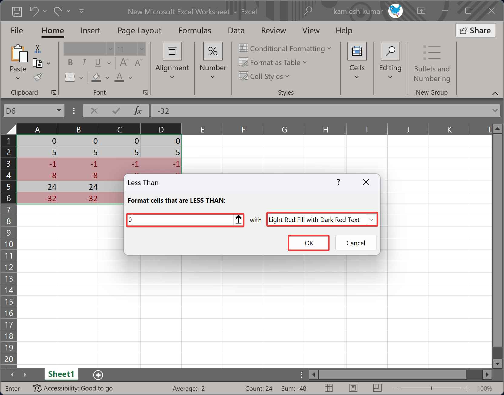
Step 6. Then, specify the value 0 in the text box.
Step 7. Finally, click the OK button to close the dialog box.
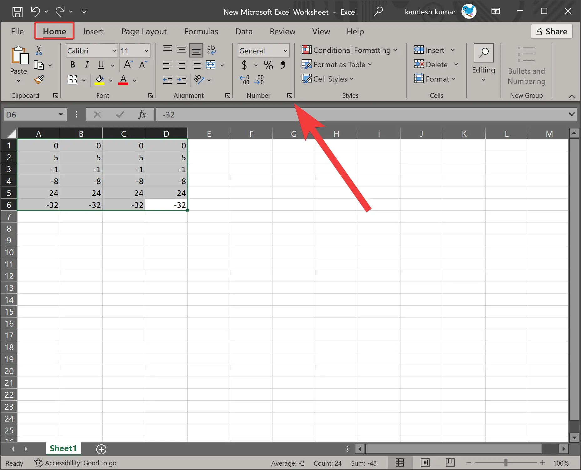
Once done, all the cells with negative numbers will turn red, while the positive numbers will remain unchanged.
How to Highlight Cells with Negative Numbers Using Custom Number Formats?
Excel allows users to create their own custom format in Excel to highlight negative numbers. Here is how to do it.
Step 1. First, choose the cells in which you want to highlight negative numbers in red.
Step 2. Then, click on the Home tab in the menu bar.
Step 3. Next, click the small arrow button under the Number group or press the keyboard shortcut Ctrl + 1 to open the Format Cells dialog box.
Step 4. Here, switch to the Number tab and select Custom on the left pane.
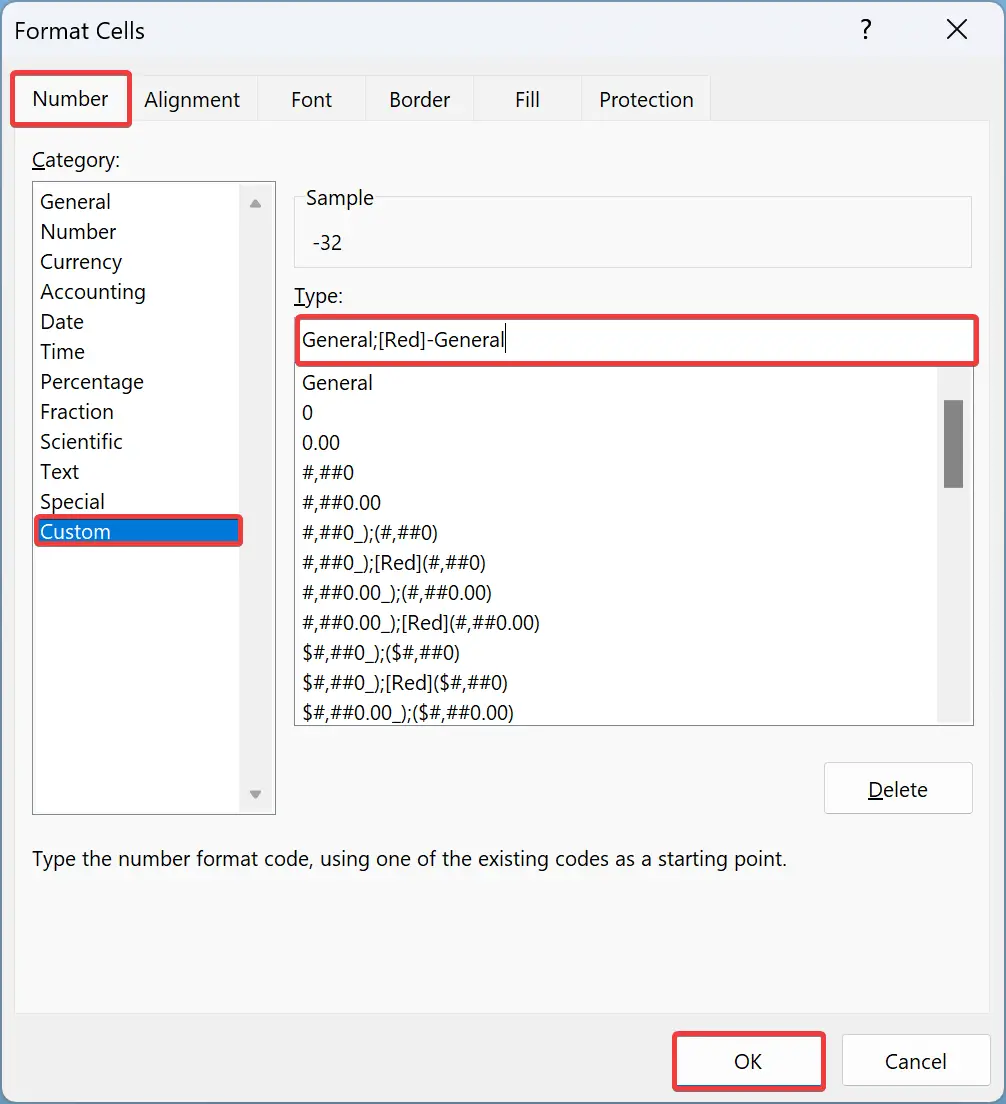
Step 5. In the “Type” box, type the following:-
General;[Red]-General
Step 6. Click the OK button.
Upon completing this process, all cells with negative numbers will turn red, while those with positive numbers will remain unchanged.
Conclusion
In conclusion, Excel’s formatting features are incredibly useful when working with data sets, and they can be used to highlight important information like negative numbers. This is especially valuable when working with financial reports that often require quick identification of losses. In this article, we learned how to highlight cells with negative values using conditional formatting and custom number formats. By using these techniques, you can easily and effectively locate negative numbers within your Excel worksheets and improve your data analysis.