Microsoft Excel is a versatile tool for data analysis and management. When working with large datasets, you may often need to extract specific information that meets certain criteria or conditions. The DSUM function, one of Excel’s database functions, is a powerful tool for precisely this purpose. In this gearupwindows article, we will explore how to use the DSUM function effectively to filter and retrieve data from a database within Excel.
What is the DSUM Function?
The DSUM function in Excel stands for “Database SUM.” It is primarily used for summing up values in a specific column of a database that meets certain criteria. This function is particularly useful when you have a large dataset, and you want to extract and summarize data based on specific conditions.
The DSUM function takes three main arguments:-
1. Database: This argument specifies the range of cells that represent the database. The database should include a header row that labels each column and subsequent rows that contain the data.
2. Field: The field argument refers to the column in the database from which you want to extract and sum data. You can identify the column by its header name or its position in the database.
3. Criteria: The criteria argument defines the conditions that the function uses to filter the data. Criteria are specified in a separate range or table with the same headers as the database. The DSUM function will sum the values in the specified field where the criteria are met.
How to Use Excel DSUM Function?
Let’s walk through a step-by-step guide on how to use the DSUM function in Excel:-
Step 1. First, make sure you have a database ready. The database should be organized in a table with a header row and data rows. Each column in the database should have a unique header that represents the type of data it contains.
Step 2. Next, create a separate table or range where you define your criteria. This criteria table should have the same headers as your database, and it will be used to filter the data.
Step 3. Choose a cell where you want the result of the DSUM function to appear. This cell will display the sum of values from your specified field based on your criteria.
Step 4. In the selected cell, type the following formula:-
=DSUM(Database, Field, Criteria)
– `Database`: Select the entire range of your database, including the header row.
– `Field`: Identify the column from your database that you want to sum. You can use either the header name or the column position.
– `Criteria`: Choose the entire criteria table or range.
Step 5. After you’ve entered the formula, press Enter. Excel will calculate the sum based on the criteria you specified, and the result will appear in the selected cell.
Example of Using DSUM Function
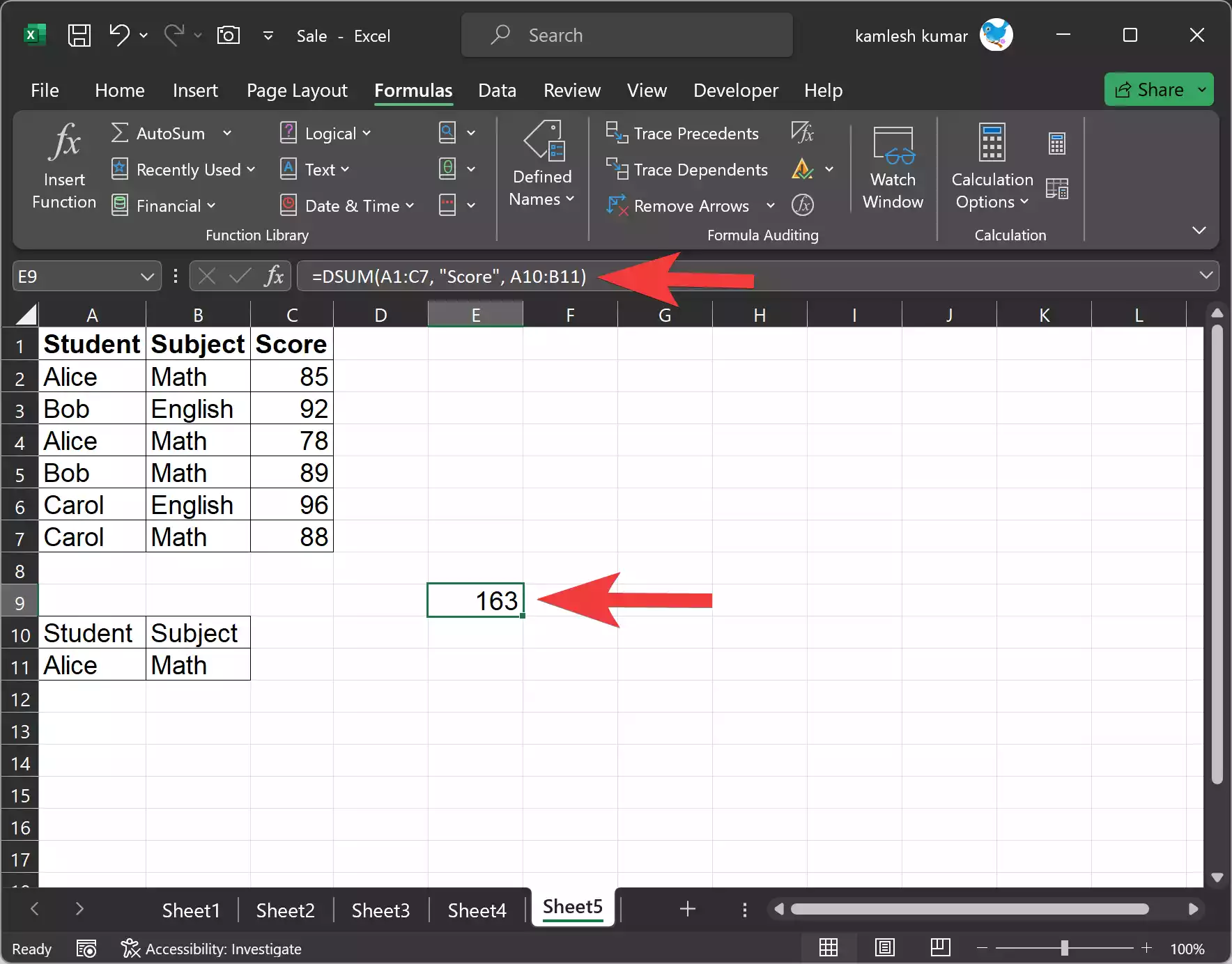
Let’s consider a practical example to better understand how the DSUM function works. Suppose you have a database of student scores with columns for “Student,” “Subject,” and “Score.” You want to find the total score for the student “Alice” in the subject “Math.”
Step 1. Set up your database and criteria table with headers that match the database columns.

Step 2. In a new cell, write the DSUM function:-
=DSUM(A1:C7, "Score", A10:B11)
– `A1:C7` is the range of your database, including the header row.
– “Score” is the field you want to sum.
– `A10:B11` is the criteria range with your specific conditions.
Step 3. Press Enter, and the result will display the total, i.e., the total score for the student “Alice” in the subject “Math.”
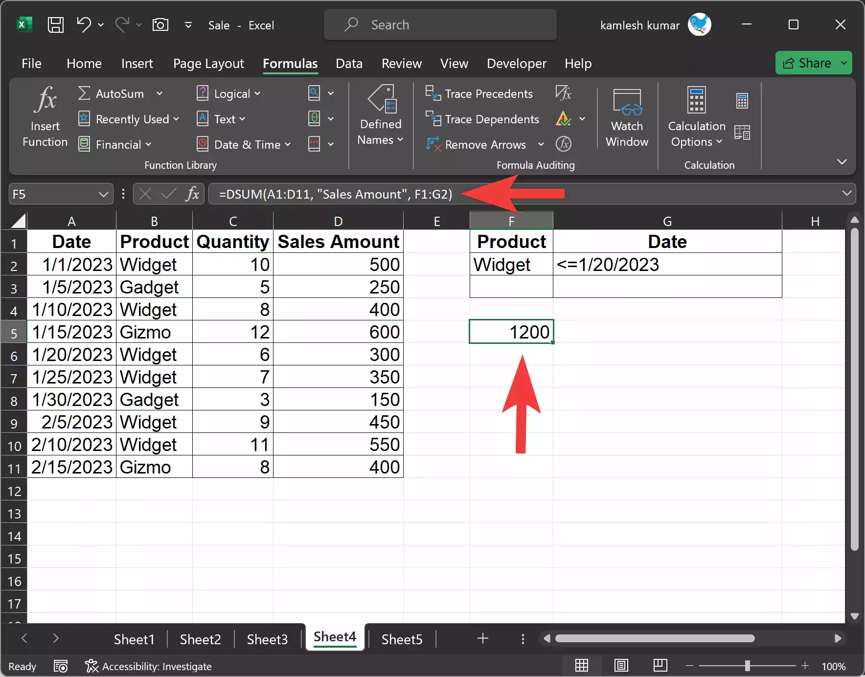
Let’s consider another practical example to better understand how the DSUM function works. Suppose you have a database of sales transactions, and you want to calculate the total sales amount for the product “Widget” sold before a specific date.
Step 1. Set up your database and criteria table with headers that match the database columns.
Step 2. In a new cell, write the DSUM function:-
=DSUM(A1:D11, "Sales Amount", F1:G2)
– `A1:D11` is the range of your database, including the header row.
– “Sales Amount” is the field you want to sum.
– `F1:G2` is the criteria range with your specific conditions.
Step 3. Press Enter, and the result will display the sum, i.e., the total Sales Amount for the product “Widget” before the date 1/20/2023.
Tips for Using DSUM Function
Here are some tips and considerations when using the DSUM function:-
1. Ensure that your database and criteria table are well-structured and organized with clear headers. This will make it easier to work with the DSUM function.
2. You can use logical operators (e.g., `<`, `>`, `<=`, `>=`, `<>`, `=`) in your criteria to filter data more precisely. For example, you can use “>=01/01/2023” to filter data on or after January 1, 2023.
3. If you want to perform multiple DSUM calculations with different criteria, you can use separate cells for each calculation.
4. Remember that the DSUM function is not case-sensitive when matching criteria.
5. Be careful with wildcards like “*” and “?” in your criteria. They may not work as expected with the DSUM function.
Conclusion
The DSUM function in Excel is a valuable tool for extracting and summarizing data from a database based on specific conditions. By structuring your database and criteria table appropriately and following the steps outlined in this article, you can harness the power of DSUM to efficiently analyze and extract valuable information from your data. Whether you’re managing sales data, inventory, or any other type of dataset, the DSUM function can help you make data-driven decisions with ease.