Microsoft Excel is a powerful spreadsheet application that allows you to perform a wide range of calculations and data analysis tasks. One common formatting requirement in Excel is the need to highlight or emphasize certain numbers within your spreadsheet. One effective way to do this is by putting a circle around a number. While Excel does not have a built-in feature specifically for drawing circles around numbers, you can achieve this effect using a combination of shapes and formatting tools available in the program. In this gearupwindows article, we will guide you through the process of putting a circle around a number in Excel.
How to Put a Circle Around a Number in Excel?
Method 1: Using Illustration
Step 1. Begin by opening the Excel spreadsheet containing the number you want to highlight with a circle. If you don’t have a spreadsheet yet, you can create a new one or use an existing one.
Step 2. Click on the cell that contains the number you want to circle. This will ensure that any shape you add will be placed precisely around that number.
Step 3. Go to the “Insert” tab in the Excel ribbon at the top of the window. Click on the Illustration button and select “Oval” or “Circle” shape. Your cursor will now turn into a crosshair.
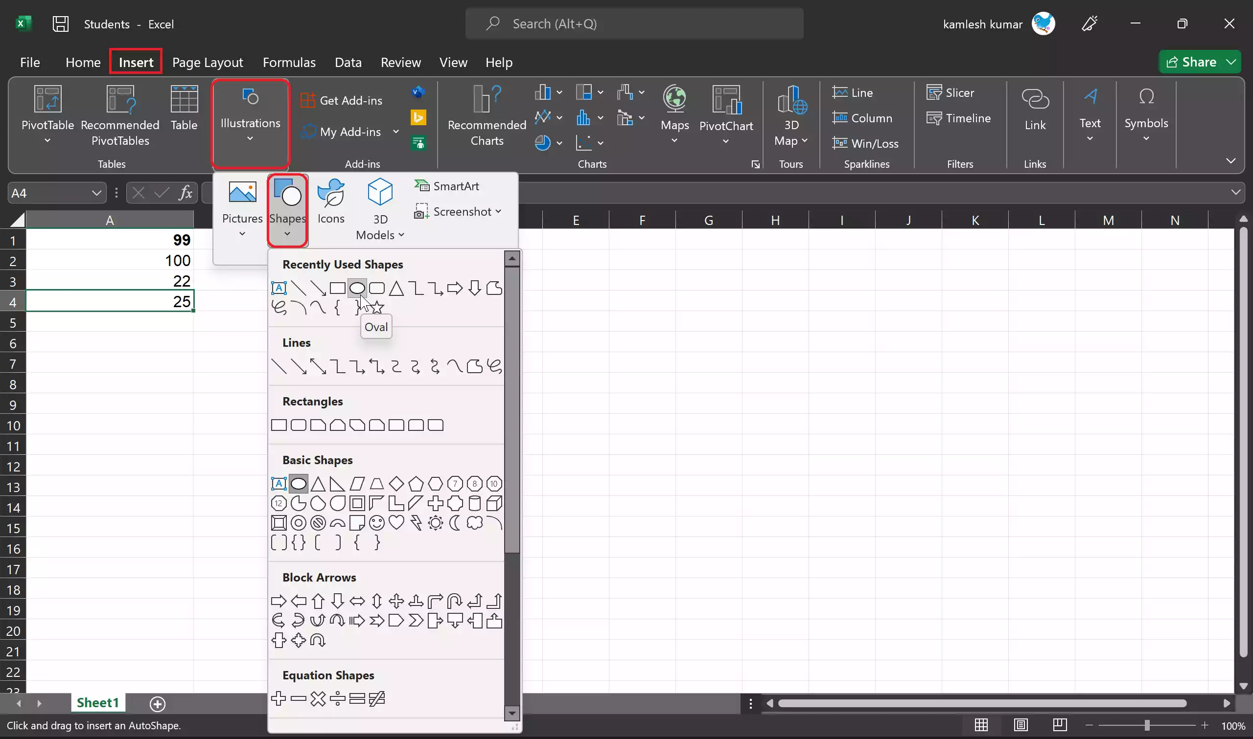
Step 4. Click and drag your mouse to draw a circle around the number in the selected cell. You can adjust the size and position of the circle as needed by clicking and dragging its handles. Make sure the circle covers the number entirely and is centered on it.
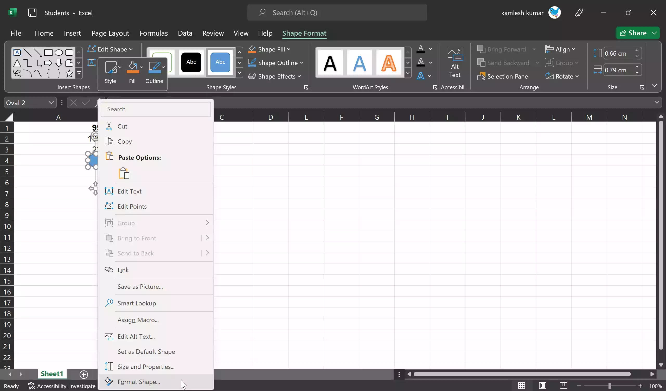
Step 5. With the circle shape selected, you can format it to make it more visually appealing or to suit your specific requirements. Right-click on the circle and choose “Format Shape” from the context menu. A Format Shape pane will appear on the right-hand side of the Excel window.
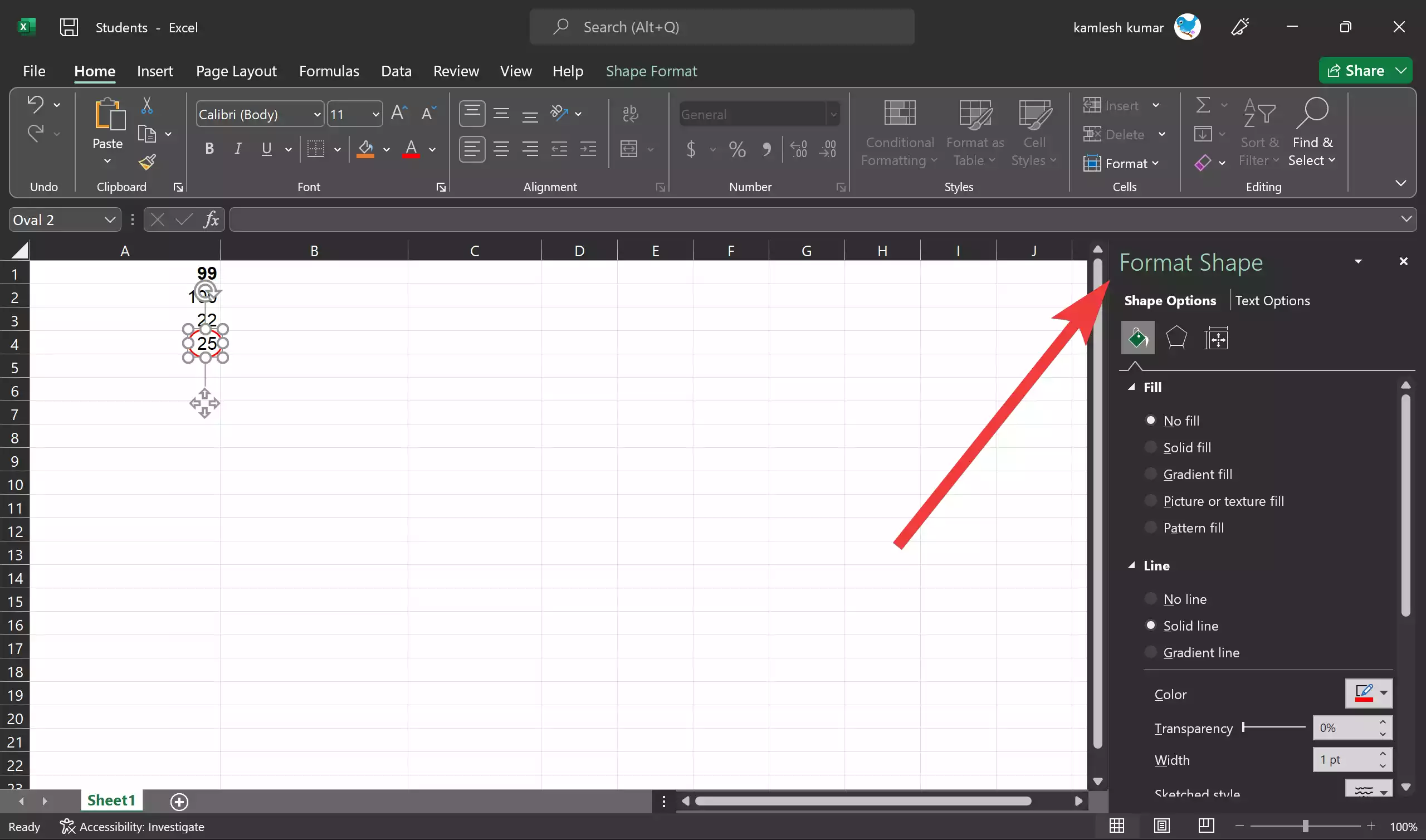
Here are some formatting options you can consider:-
- Line Color: You can change the color of the circle’s outline by selecting a different color under the “Line” option in the Format Shape pane.
- Line Style: Adjust the thickness and style of the circle’s outline by modifying the “Line Style” settings.
- Fill Color: You can fill the circle with a color by choosing a fill color under the “Fill” option. This can help the circle stand out more.
- Effects: Explore other effects, such as shadows or 3D formatting, to make the circle visually appealing.
Step 6. If the circle is not perfectly centered on the number or if you want to fine-tune its position, you can click and drag it to the desired location. Excel will help you align it using guidelines that appear as you move the shape.
Step 7. Finally, don’t forget to save your Excel spreadsheet to preserve the circle around the number you’ve highlighted.
Method 2: Using Symbol
Another method to put a circle around a number in Excel involves using symbols. This method allows you to insert a circle symbol around the desired number. Here’s a step-by-step guide:-
Step 1. Launch Microsoft Excel and open the spreadsheet containing the number you want to highlight with a circle.
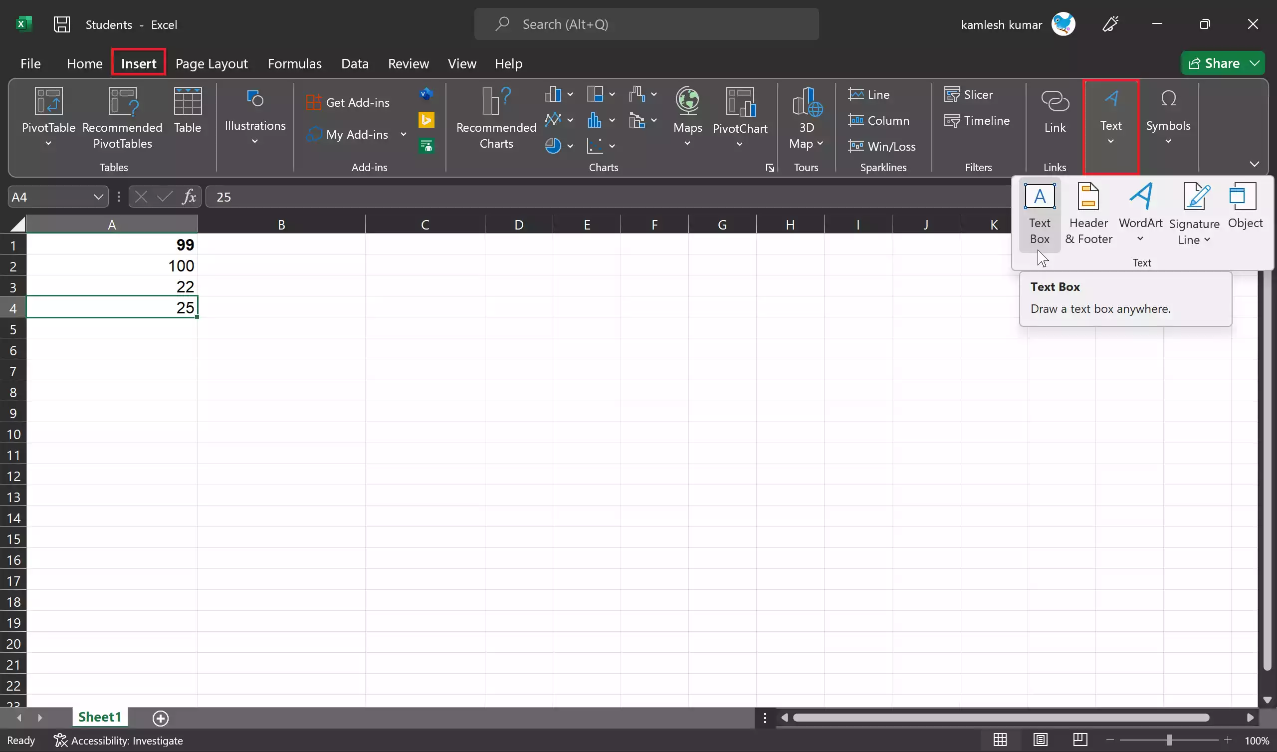
Step 2. Go to the “Insert” tab in the Excel ribbon. Click on the “Text” button, select “Text Box” in the Text group, and then draw a text box on the spreadsheet where you want to place the circled number.
Quick Note: To make it clearer, you can draw a text box in a blank space in a spreadsheet. Later, you can move this text box to cover the number.
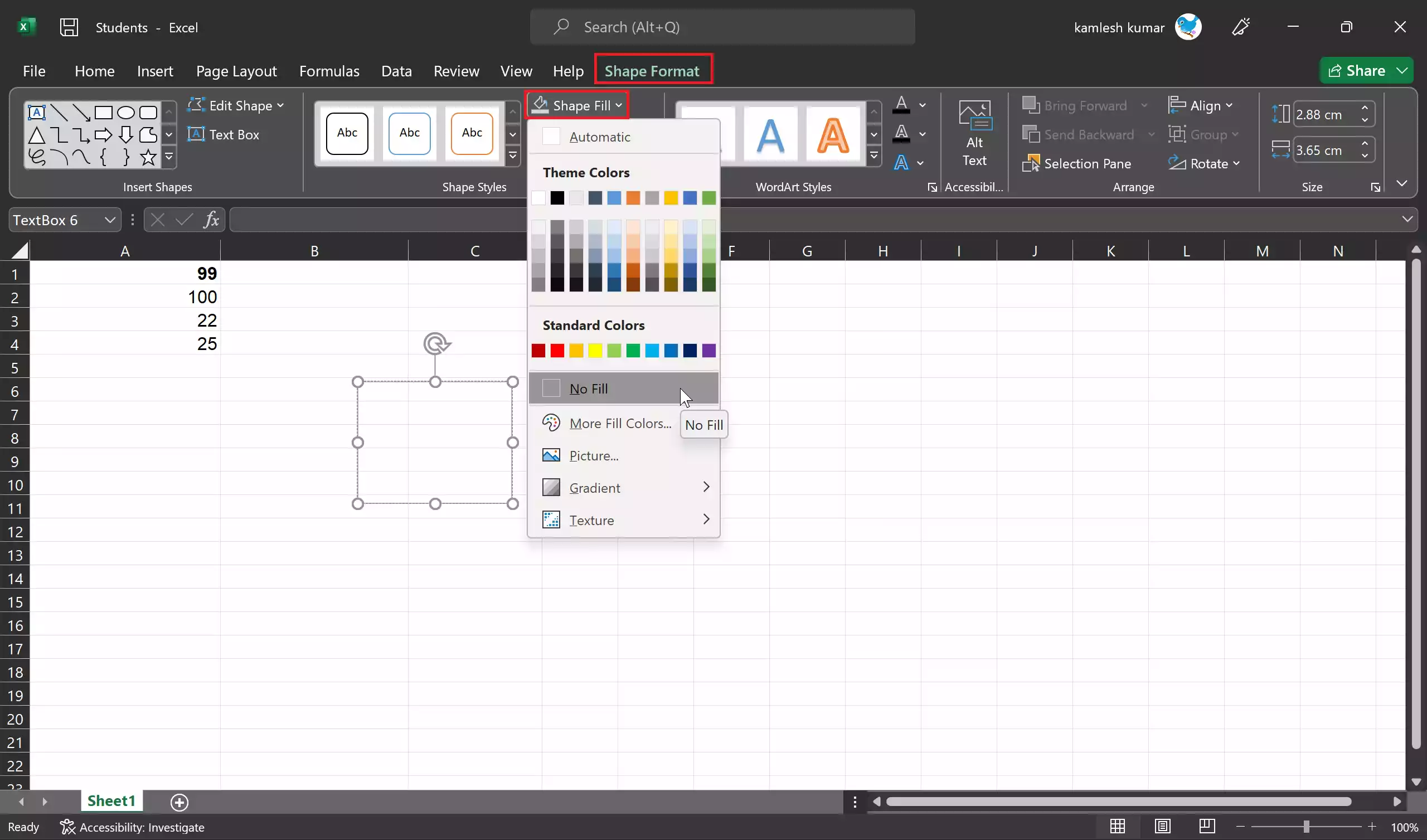
Step 3. Select the text box you created, and then go to the “Shape Format” tab in the ribbon. Click on the “Shape Fill” button and choose “No Fill” to make the text box transparent.
Step 4. Double-click the text box to enter text-editing mode.
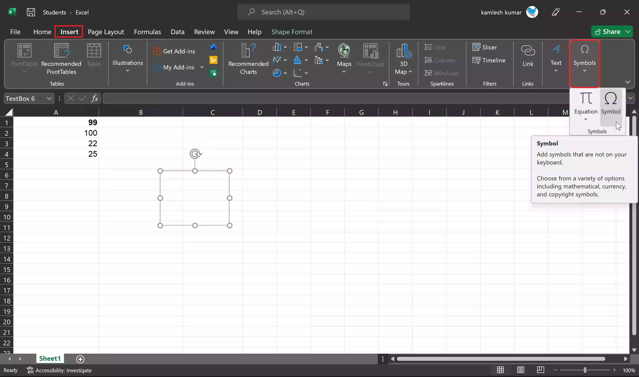
Step 5. Go back to the “Insert” tab and click on the “Symbols” button. From the dropdown menu, select “Symbol.”
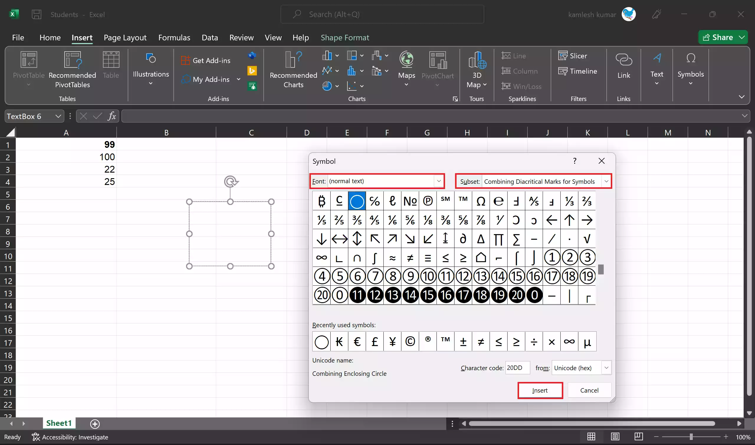
Step 6. A Symbol dialog box will appear. In this dialog box:-
- Click the “Font” dropdown and select “(Normal Text).”
- In the “Subset” dropdown, choose “Combining Diacritical Marks for Symbols.”
- Scroll through the list of symbols and select the circle symbol.
- Click the “Insert” button. The circle symbol will be inserted into the text box.
Step 7. Position the text box with the circle symbol over the number you want to highlight. You can click and drag the text box to place it accurately.
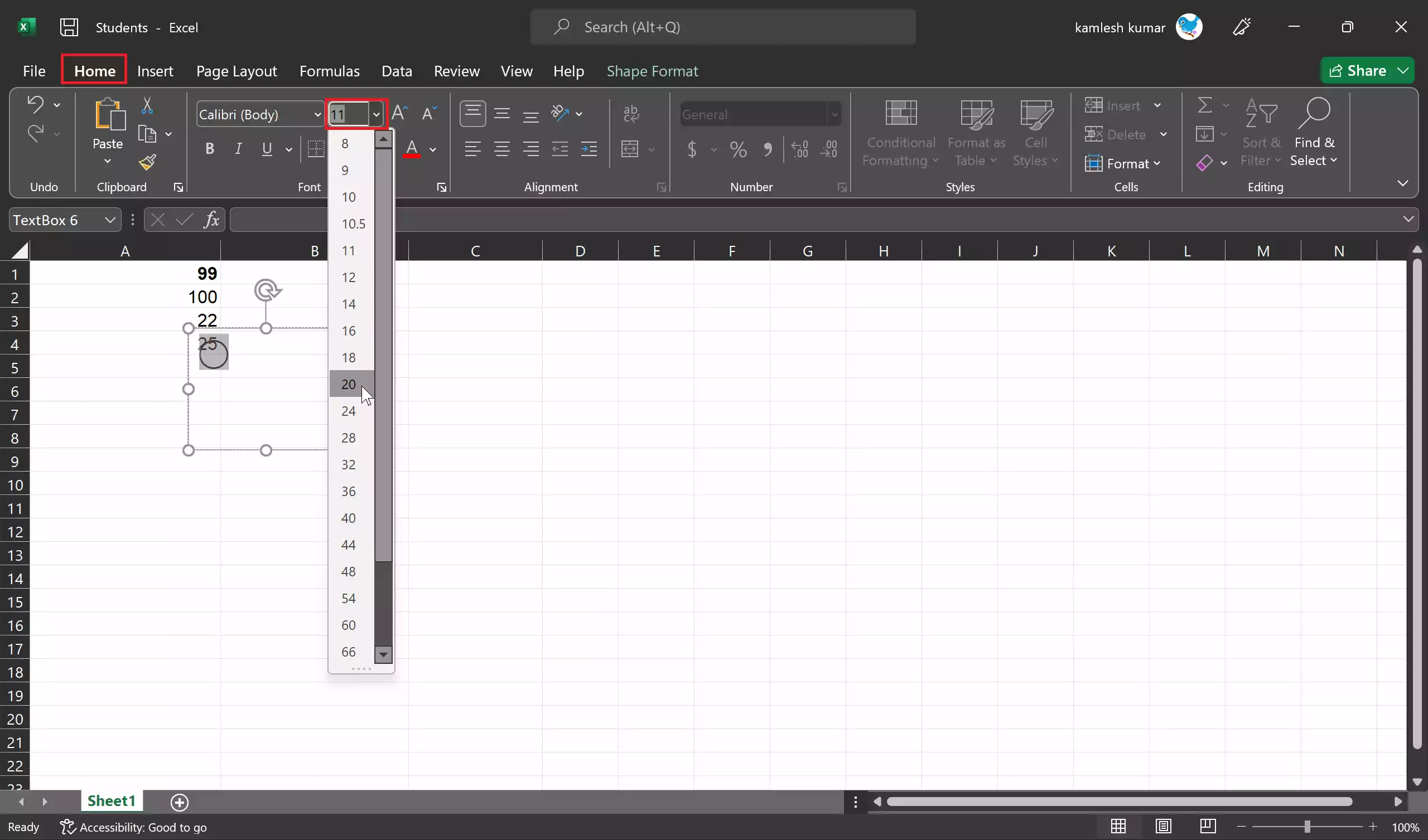
Step 8. If you want to change the size of the circle symbol, click on the symbol inside the text box to select it. Then, go to the “Home” tab, and in the “Font Size” dropdown, select the desired size for the circle symbol.
Step 9. To remove the outline around the text box, select the text box containing the circle symbol. Go to the “Shape Format” tab in the ribbon, click on “Shape Outline,” and choose “No Outline.”
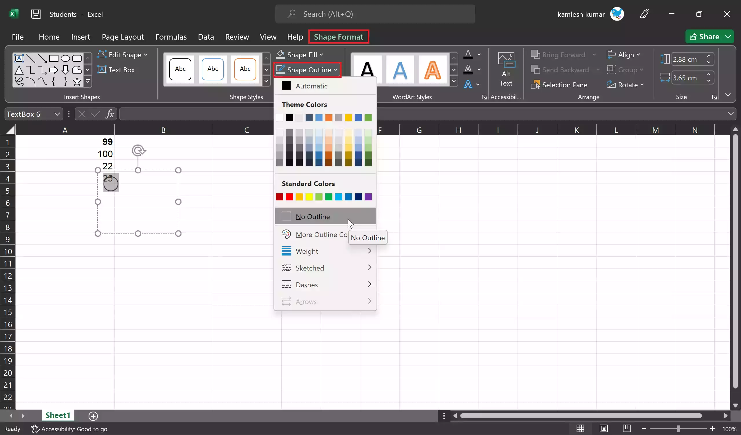
The outline around the text box will disappear, leaving just the circled number. This method provides a visually effective way to highlight specific numbers in your Excel spreadsheet using symbols and text boxes.
Method 3: Using Excel Add-Ins
There are several Excel add-ins available that provide advanced formatting options, including the ability to add circles or shapes around numbers. Some popular add-ins include “Kutools for Excel” and “AbleBits Ultimate Suite.” These tools often have dedicated features for adding shapes around data points, making it easier to achieve the desired effect.
Conclusion
In conclusion, Microsoft Excel offers multiple methods for highlighting and emphasizing numbers within your spreadsheet, including putting a circle around them. Whether you prefer using illustration tools, symbols, or Excel add-ins, you have the flexibility to choose the method that best suits your needs and preferences. By following the steps outlined in this guide, you can effectively enhance the visual presentation of your data in Excel, making it easier to convey important information and insights.