Microsoft Excel is a powerful spreadsheet application that offers a wide array of functions to help you manipulate and analyze your data. One of these functions is the FILTER function, introduced in Excel 365 and Excel 2019. The FILTER function is particularly useful for extracting specific data from a larger dataset based on user-defined criteria. In this gearupwindows article, we’ll explore how to use the FILTER function in Microsoft Excel, step by step.
Understanding the FILTER Function
The FILTER function in Excel is designed to retrieve specific records from a dataset that meet certain criteria or conditions. This makes it invaluable when you want to filter, sort, or analyze data without manually sifting through your dataset. The FILTER function takes an array of data as input and returns a filtered array, adhering to the specified conditions. Its syntax is as follows:
=FILTER(array, include, [if_empty])
– `array`: This is the range of data you want to filter. It can be a column, row, or a combination of both.
– `include`: This argument is used to specify the conditions or criteria for filtering. The criteria are applied to each row in the array.
– `[if_empty]` (optional): You can specify a value to display if no results meet the specified criteria. If left blank, it defaults to an empty cell.
How to Use FILTER Function in Microsoft Excel?
Now, let’s dive into how to use the FILTER function in Excel.
Step 1. Begin by opening Microsoft Excel and loading your dataset. Ensure that your data is organized in columns and rows, with headers for each column, making it easier to work with the FILTER function.
Step 2. Select the cell where you want the filtered data to appear. This will be the cell where you enter the FILTER function.
Step 3. In the selected cell, type `=FILTER(` to start the FILTER function. Now, you need to specify the array.
Step 4. Click and drag to select the range of data you want to filter. Alternatively, you can manually type the range or use the range selector to highlight the data. This range should contain both the column headers and the data you want to filter.
For example, if you have your data in cells A1 to B10, you would enter `A1:B10` as the array. Now, the formula will look like something =FILTER(A1:B10,
Step 5. After specifying the array, add a comma to move on to the next argument. Here, you define the criteria you want to apply to your data. This can be a logical expression, a formula, or a reference to another cell.
For this example, we want to filter products with prices higher than $1, so we’ll define the criteria. Enter:-
=FILTER(A1:B10, B1:B10 > 1,
You can also use logical operators like `AND` and `OR` to create complex criteria.
Step 6. Close the function by adding a closing parenthesis, `)`, and press Enter. The selected cell will now display the filtered results based on the criteria you defined.
The formula should now look like this:-
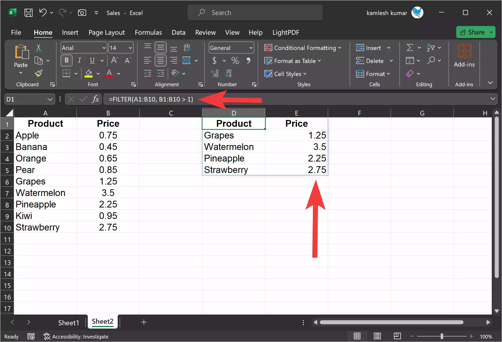
=FILTER(A1:B10, B1:B10 > 1)
Step 7. If you wish, you can add an optional `[if_empty]` argument to specify what should appear in the selected cell if there are no matches based on your criteria. If you leave it empty, the cell will display nothing when no matches are found.
Excel will display only the products with prices higher than $1 in the specified cell. This is a simple example, but you can use more complex criteria to filter data in real-world scenarios.
Tips for Using the FILTER Function Effectively
- Use Absolute Cell References: When creating complex criteria for the FILTER function, it’s a good practice to use absolute cell references. This ensures that your criteria remain the same when you copy the formula to other cells.
- Combine FILTER with Other Functions: You can combine the FILTER function with other Excel functions like SORT, UNIQUE, and SUM to perform more advanced data analysis and reporting.
- Use Named Ranges: If your data is spread across multiple sheets or workbooks, consider defining named ranges to make it easier to work with the FILTER function.
- Keep Your Data Clean: Ensure your data is consistent and free of errors, as filtering relies on the accuracy and integrity of your data.
- Test Your Criteria: Before applying the FILTER function to large datasets, test your criteria on a smaller subset to make sure you are getting the desired results.
Conclusion
In conclusion, the FILTER function in Microsoft Excel is a powerful tool for efficiently extracting specific data from your spreadsheets. By understanding its syntax and following these step-by-step instructions, you can streamline your data analysis and reporting tasks, saving time and reducing the risk of errors. Whether you are working with financial data, sales reports, or any other type of dataset, the FILTER function can help you make informed decisions and gain valuable insights from your data.
