Microsoft Excel is a powerful spreadsheet application that offers a multitude of features to help users organize and analyze data. One common task you might need to perform is shifting cells down in Excel, which involves moving the contents of one or more cells to a lower position within your worksheet. This can be useful for various purposes, such as reorganizing data or making room for new information. In this gearupwindows article, we will explore various methods for shifting cells down in Excel.
How to Shift Cells Down in Excel?
Method 1: Using Cut and Paste
The most straightforward way to shift cells down in Excel is by using the cut and paste method. Here’s how to do it:-
Step 1. Select the Cells: First, select the cells that you want to shift down. You can click and drag your mouse to highlight the range, or you can hold down the Shift key while using the arrow keys to select cells.
Step 2. Cut the Cells: Right-click on the selected cells and choose “Cut” from the context menu, or use the keyboard shortcut `Ctrl+X` (or `Cmd+X` on a Mac).
Step 3. Select the Destination: Click on the cell where you want to move the cut cells. This is the new position for your data.
Step 4. Paste the Cells: Right-click in the destination cell and select “Insert Cut Cells” from the context menu, or use the keyboard shortcut `Ctrl+V` (or `Cmd+V` on a Mac). The cut cells will be pasted into the new location, shifting the existing data downwards.
Method 2: Using the Drag-and-Drop Method
Another simple way to shift cells down is by using the drag-and-drop method. Here’s how it works:-
Step 1. Select the Cells: Start by selecting the cells you want to shift. As before, you can click and drag your mouse to highlight the range.
Step 2. Move the Mouse Pointer: Hover your mouse pointer over the border of the selected cells. The pointer will change to a four-sided arrow.
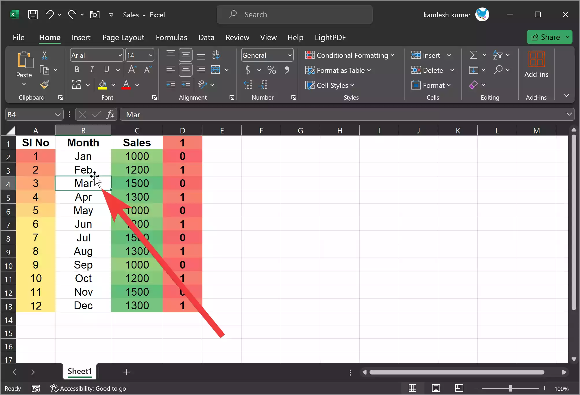
Step 3. Drag and Drop: Click and drag the selected cells to the new location within the worksheet. When you release the mouse button, the cells will be moved to the new position.
Method 3: Using the “Insert” Feature
Excel provides an “Insert” feature that allows you to add rows or columns, effectively shifting the cells down. Here’s how to use it:-
Step 1. Select the Row: Click on the row below where you want to insert new cells.
Step 2. Right-click on the Row: On the selected row, right-click and choose the “Insert” option.
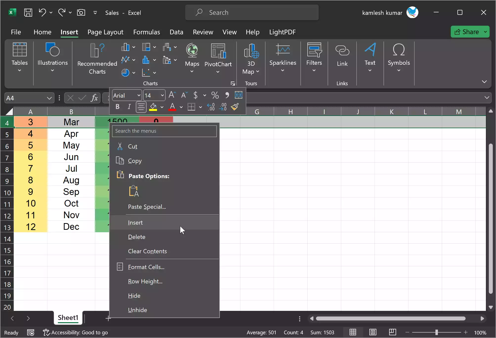
This action will push the row below downward, making room for your new data.
Method 4: Using Excel Functions
If you need to shift cells down based on certain conditions or calculations, you can use Excel functions like OFFSET or INDIRECT. These functions allow you to dynamically reposition data. For example, you can use the OFFSET function to reference a cell relative to another cell and then use this result in calculations or data organization.
Here’s an example using the OFFSET function:-
Step 1. Select a Destination Cell: Start by selecting the cell where you want to display the shifted data.
Step 2. Use the OFFSET Function: In the formula bar, type a formula using OFFSET to reference the original cell whose contents you want to shift. For instance, if you want to shift cell A1 down, you could use the formula `=OFFSET(A1,1,0)` to reference the cell one row below.

Step 3. Press Enter: After entering the formula, press Enter to display the result, which will be the content of the cell you want to shift.
These are some of the methods you can use to shift cells down in Excel. The method you choose will depend on your specific needs and preferences. Whether you opt for the simplicity of cut and paste, the intuitive drag-and-drop method, the convenience of Excel’s “Insert” feature, or the flexibility of Excel functions, Excel provides a solution for every data-shifting scenario. By mastering these techniques, you’ll be better equipped to organize and manipulate your data efficiently in Excel.
