Microsoft Excel is a powerful tool for data analysis and manipulation, and it provides various functions that can help you extract and transform data with ease. Two such functions are TAKE and DROP, which are particularly useful when you need to work with large datasets or filter specific portions of your data. In this article, we will explore how to use the TAKE and DROP functions in Excel, along with examples to illustrate their practical applications.
Note: The TAKE and DROP function is only supported in Excel for Microsoft 365 (Windows and Mac) and Excel for the web. In earlier Excel versions, you can use an OFFSET formula instead TAKE function.
Understanding the TAKE and DROP Functions
The TAKE and DROP functions in Excel are designed to help you extract or exclude specific rows from a range of data. These functions are often used in conjunction with other Excel functions, such as IF, SUM, or AVERAGE, to perform more complex data analysis tasks.
- TAKE Function: The TAKE function allows you to extract a specified number of rows from the beginning of a dataset. It is helpful when you want to focus on a subset of data without removing the original data.
- DROP Function: The DROP function, on the other hand, helps you skip a specified number of rows from the beginning of a dataset, effectively excluding them from your analysis. This function is useful when you want to disregard certain initial rows of data.
Syntax of the TAKE and DROP Functions
Before diving into examples, let’s understand the syntax of these functions:-
TAKE Function Syntax
=TAKE(range, count)
- range: This is the range of cells or data from which you want to extract rows.
- count: This parameter specifies the number of rows to take from the beginning of the range.
DROP Function Syntax
=DROP(range, count)
- range: The range of cells or data from which you want to skip rows.
- count: This parameter specifies the number of rows to skip from the beginning of the range.
Practical Examples
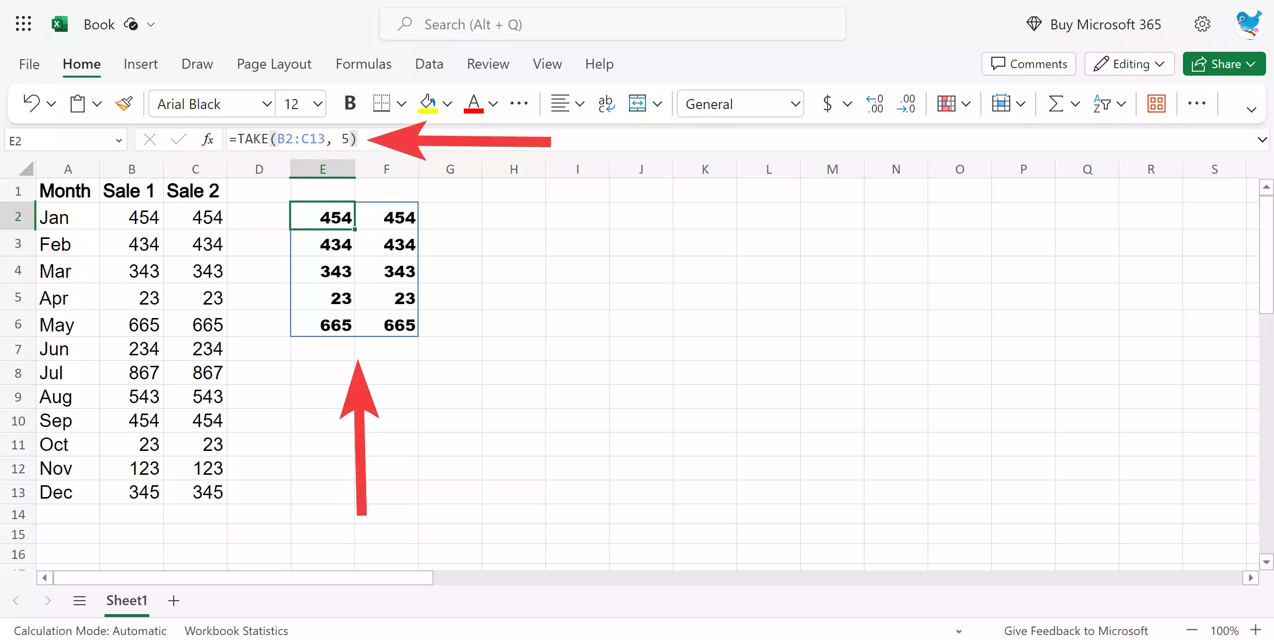
Example 1: Using the TAKE Function
Suppose you have a dataset of monthly sales figures and you want to analyze the first 5 months’ data. You can use the TAKE function for this purpose.
=TAKE(B2:C13, 5)
In this example:-
- `B2:C13` represents the range of your data containing 12 months of sales figures.
- `5` is the count parameter, indicating that you want to extract the first 5 rows from the range.
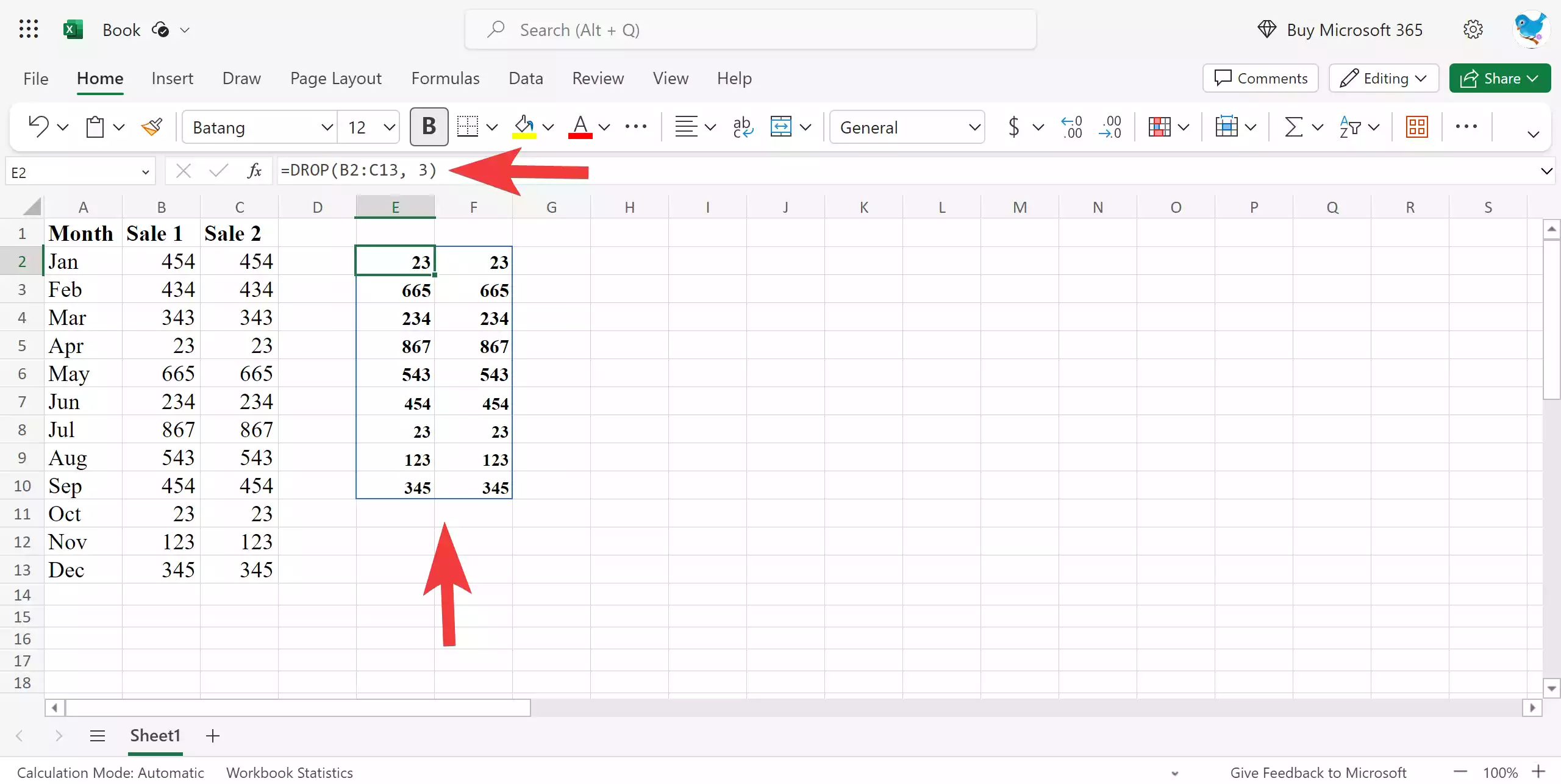
Example 2: Using the DROP Function
Let’s say you have a list of monthly sales figures, but the first 3 rows are headers and not actual sales. You can use the DROP function to exclude these header rows.
=DROP(B2:C13, 3)
In this example:-
- `B2:C13` is the range containing monthly sales.
- `3` is the count parameter, specifying that you want to skip the first 3 rows.
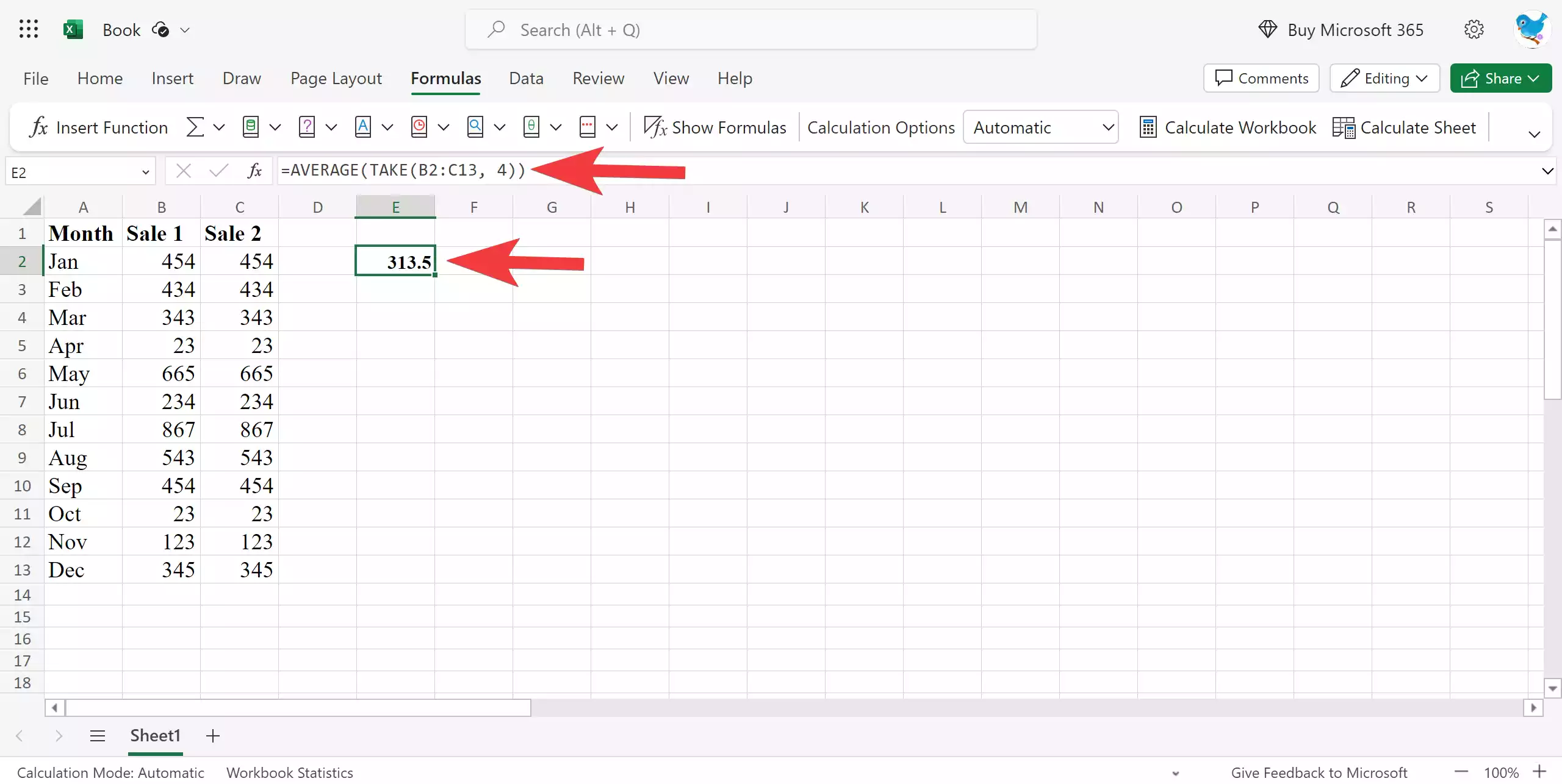
Combining with Other Functions
Both the TAKE and DROP functions can be combined with other Excel functions for more advanced data analysis. Here’s an example that demonstrates how to use the TAKE function along with the AVERAGE function:-
Suppose you have a dataset of monthly sales, and you want to calculate the average sales of the first 4 monthly sales.
=AVERAGE(TAKE(B2:C13, 4))
In this case:-
- `B2:C13` represents the range containing test scores.
- `4` specifies that you want to take the first 4 rows from the range.
- `AVERAGE` is used to calculate the average of these selected values.
Conclusion
The TAKE and DROP functions in Excel are powerful tools for manipulating and extracting data from ranges. Whether you need to focus on specific subsets of data or exclude certain rows from your analysis, these functions can save you time and simplify your data processing tasks. By understanding their syntax and applying them in combination with other Excel functions, you can unlock the full potential of Excel for data analysis and reporting.