Microsoft Excel is a powerful spreadsheet tool that is widely used for data analysis and presentation. One common task in Excel is to enhance the readability and aesthetics of your data by applying colors to alternate rows. This technique makes it easier to follow and interpret data, especially in large spreadsheets. In this article, we will explore various methods to apply color to alternate rows in Excel, catering to different versions of the software.
Why Apply Color to Alternate Rows?
Coloring alternate rows in an Excel spreadsheet serves several practical purposes:-
- Improved Readability: Applying colors to alternate rows makes it easier for readers to distinguish one row from another, which can be especially helpful when working with large datasets.
- Enhanced Focus: When you’re dealing with a large amount of data, applying colors to alternate rows helps maintain focus on the current line of data and reduces the chance of data entry errors.
- Visual Appeal: Adding color to your spreadsheet not only improves functionality but also enhances the overall visual appeal of your documents.
Now, let’s delve into the methods of applying color to alternate rows in Excel.
How to Apply Color to Alternate Rows in Microsoft Excel?
Method 1: Conditional Formatting (Excel 2007 and Later)
Conditional formatting is a powerful feature in Excel that allows you to apply formatting rules based on specific conditions. This method is available in Excel 2007 and later versions.
Step 1. Select the range of cells where you want to apply the alternate row colors.
Step 2. Go to the “Home” tab on the Excel ribbon.
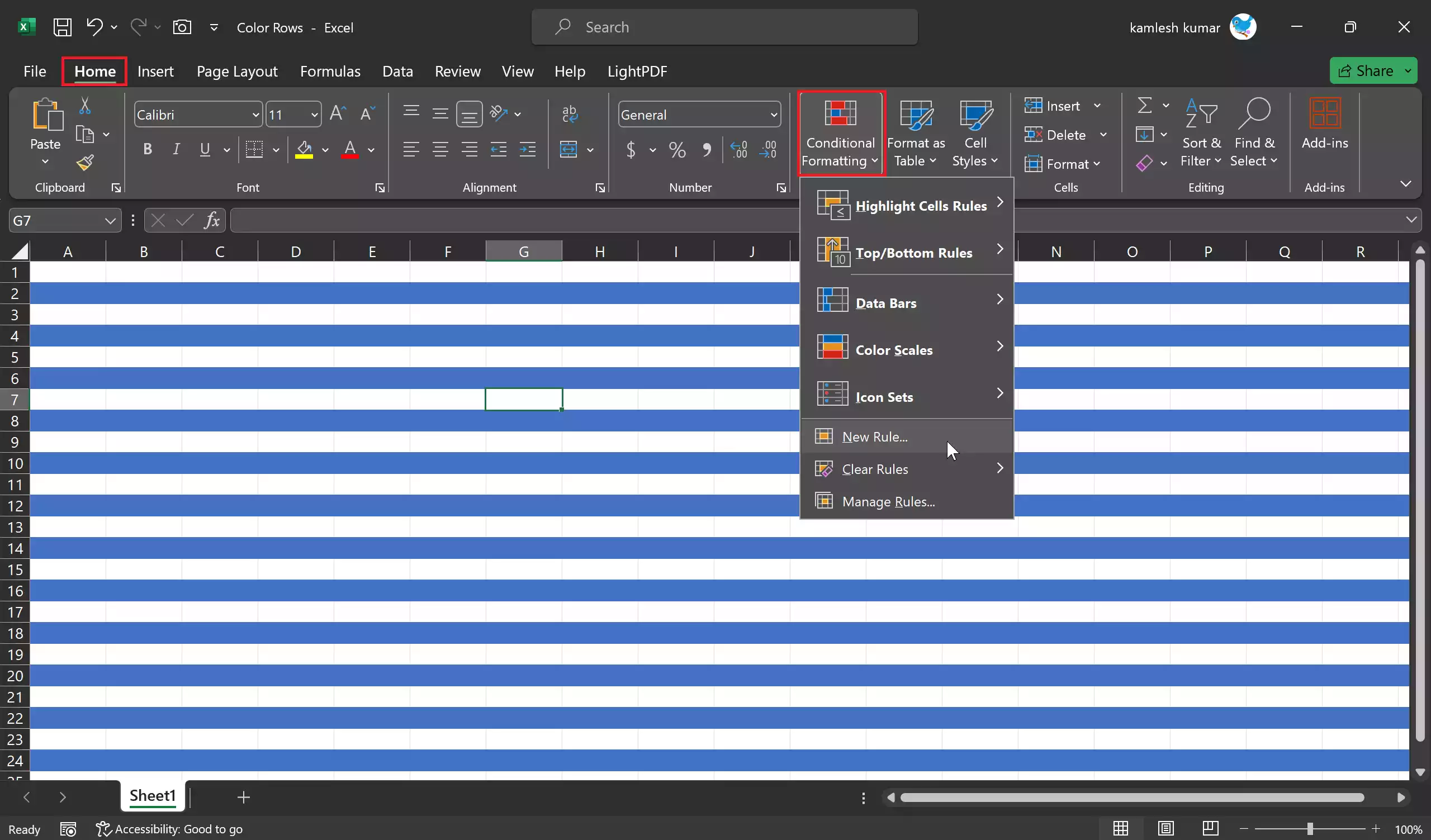
Step 3. In the “Styles” group, click on “Conditional Formatting.”
Step 4. Choose “New Rule.”
Step 5. In the “New Formatting Rule” dialog box, select “Use a formula to determine which cells to format.”

Step 6. Enter the following formula:-
=MOD(ROW(),2)=0
This formula checks if the row number is even (for alternate rows).
Step 7. Click on the “Format” button to choose the fill color you want for the alternate rows.
Step 8. Select your desired color from the “Fill” tab in the “Format Cells” dialog. After selecting your color, click “OK.”

Step 9. Click “OK” again in the “New Formatting Rule” dialog box.
Now, the alternate rows in your selected range will be color-coded.
Method 2: Excel Tables (Excel 2013 and Later)
If you are using Excel 2013 or a later version, you can leverage Excel tables to apply color to alternate rows automatically.
Step 1. Select the range of cells you want to format.
Step 2. Go to the “Insert” tab on the Excel ribbon.

Step 3. Click on “Table.” Excel will ask if your table has headers. Make sure the box is checked if your data has headers, and uncheck it if not.
Step 4. In the “Create Table” dialog box, make sure that the “My table has headers” option is correctly set, and choose a table style. Click “OK.”
Step 5. Excel will convert your selected range into a table format. By default, alternate row shading is applied automatically, which you can further customize in the “Table Design” tab that appears.

Method 3: Color Scales (Excel 2010 and Later)
In Excel 2010 and later versions, you can apply color scales to alternate rows by using conditional formatting. This method allows you to create a gradient effect on the selected range.
Step 1. Select the range you want to format.
Step 2. Go to the “Home” tab on the Excel ribbon.
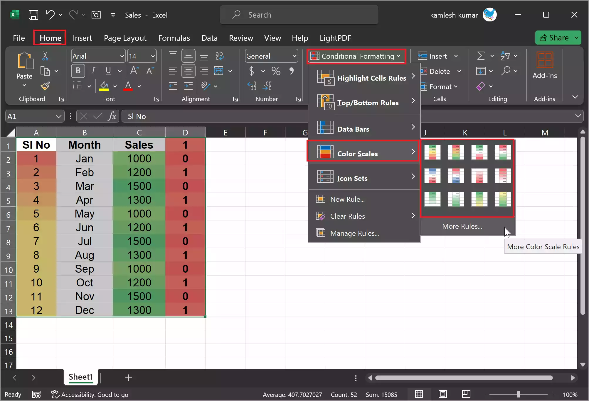
Step 3. In the “Styles” group, click on “Conditional Formatting.”
Step 4. Choose “Color Scales” and pick one of the predefined color scales.
Step 5. Adjust the color scale options as desired and click “OK.”
Now, Excel will apply the color scale to the selected range, providing a visual distinction between alternate rows.
Conclusion
In conclusion, Microsoft Excel offers various methods to enhance the readability and aesthetics of your data by applying colors to alternate rows. This technique not only improves data interpretation, especially in large spreadsheets, but also aids in maintaining focus and enhances the visual appeal of your documents. Whether through conditional formatting, Excel tables, or color scales, Excel provides versatile tools to make your data more visually engaging and easier to work with.
