Microsoft Excel is a powerful spreadsheet software that is widely used for data analysis, calculations, and creating charts and graphs. While Excel is primarily known for its number-crunching capabilities, it also offers some handy features for handling visual elements, such as capturing screenshots. In this article, we will explore how to capture screenshots within Excel, making it easier to document your work and enhance your data presentations.
Why Capture Screenshots in Excel?
Capturing screenshots within Excel can be incredibly useful for several reasons:-
- Documentation: Screenshots allow you to document your work, making it easier to reference specific data, formulas, or charts in the future.
- Communication: Screenshots are an effective way to share information and data with others, especially when you want to highlight particular aspects of your spreadsheet.
- Presentation: If you’re creating reports or presentations in Excel, inserting screenshots can help illustrate your points and make your work more visually appealing.
- Troubleshooting: When seeking help or troubleshooting issues in Excel, screenshots can provide a clear visual representation of the problem you’re encountering.
Now, let’s delve into the step-by-step process of capturing screenshots with Excel.
How to Capture Screenshots With Excel?
To capture Screenshots with Excel, use these steps:-
Step 1. Begin by launching Microsoft Excel and opening the spreadsheet where you want to capture and insert screenshots.
Step 2. Arrange your Excel window and any other applications or windows you want to capture so that they are visible on your screen. Ensure that the content you want to capture is in the foreground.
Step 3. Click on the “Insert” tab in the Excel Ribbon. This tab is typically located in the top menu bar.
Step 4. In the “Illustrations” group, look for the “Screenshot” button. It may also be labeled as “Screenshot and Screen Clipping.”
Step 5. Click on the “Screenshot” button to reveal a dropdown menu displaying the available screenshot options.
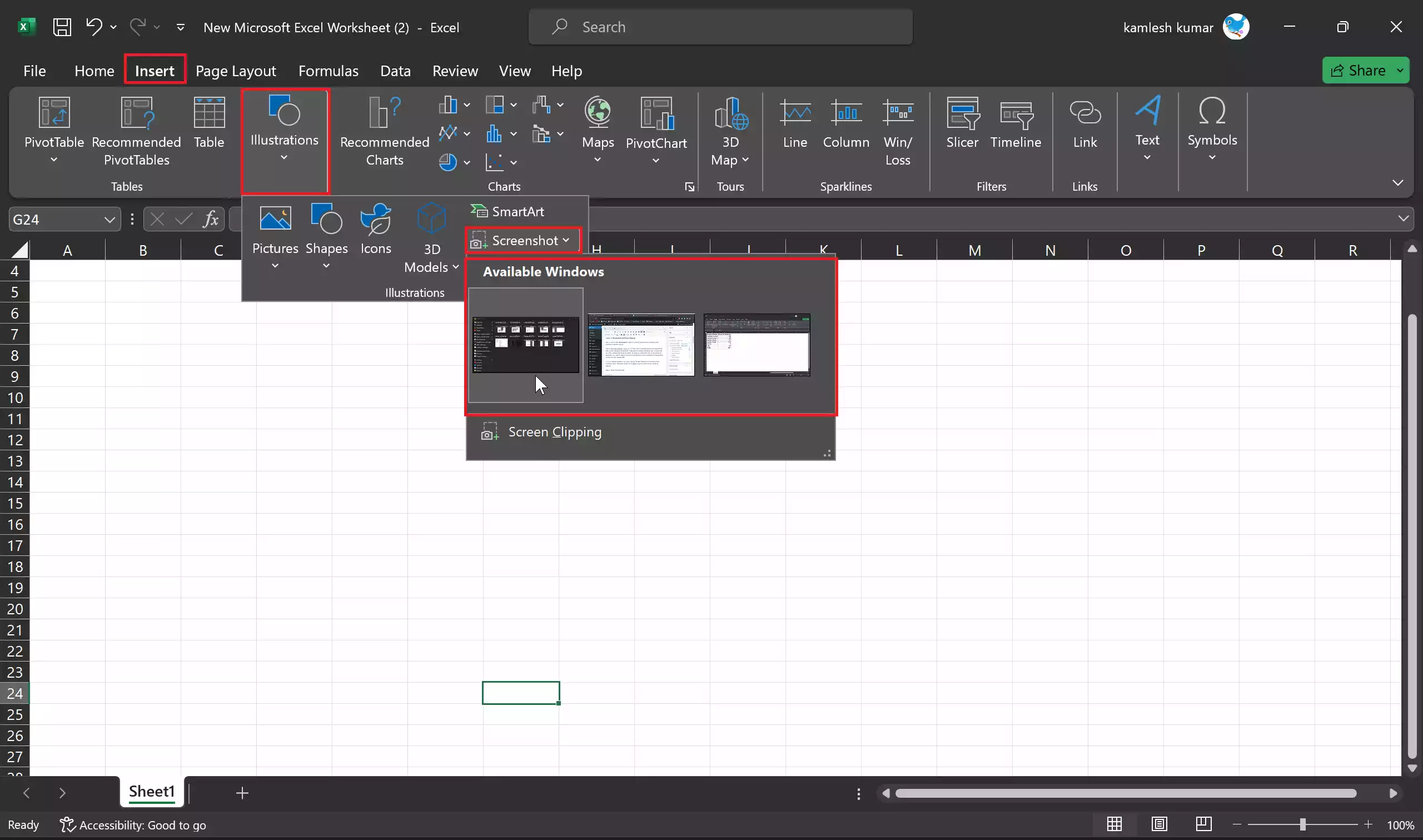
Step 6. From the dropdown menu, you will see a list of available windows and applications that you can capture as screenshots. These options typically include all open windows and any other windows that Excel can detect. To capture a screenshot, click on the window or application you want to capture. Excel will automatically insert a screenshot of the selected window into your spreadsheet.
Step 7. If your desired window is not listed, click on “Screen Clipping” at the bottom of the dropdown menu. This option allows you to select a specific portion of your screen to capture.
Step 8. Press and hold the left mouse button to capture the desired portion of activate window.
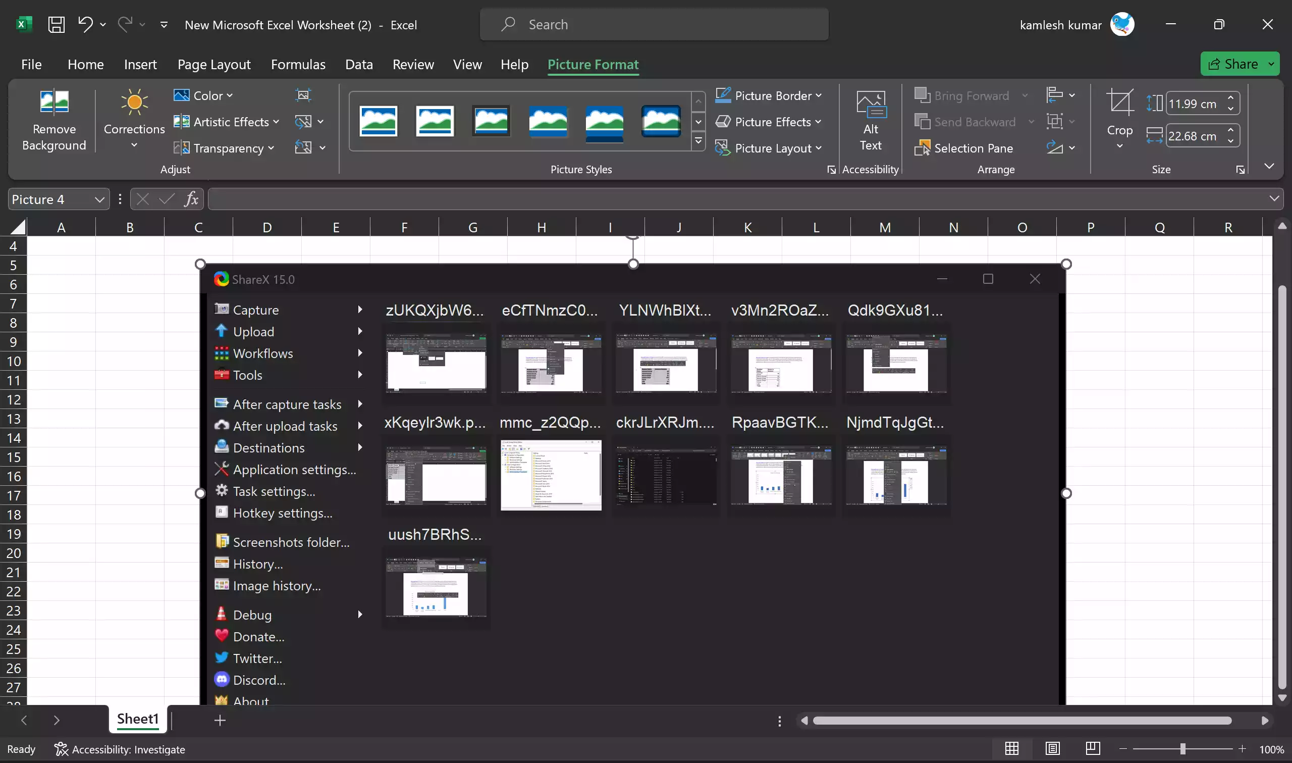
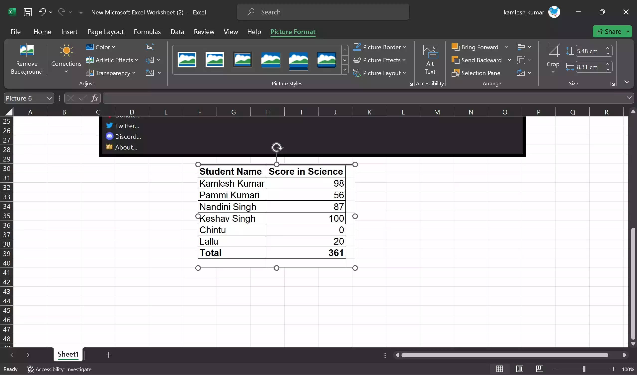
Step 9. After capturing the screenshot, Excel will automatically insert it into your spreadsheet at the location of your cursor. You can then resize and format the screenshot as needed to fit your document’s requirements.
Step 10. Don’t forget to save your Excel spreadsheet after inserting the screenshot to preserve your work.
How to Add Excel Camera to Quick Access Toolbar?
If you want to use Excel Camera frequently, you might prefer to add it to Quick Access Toolbar:-
Step 1. Begin by launching Microsoft Excel and opening the workbook where you want to add the Excel Camera to the Quick Access Toolbar.
Step 2. To customize it, click on the small down arrow (or customize icon) at the right end of the QAT. This opens a dropdown menu.
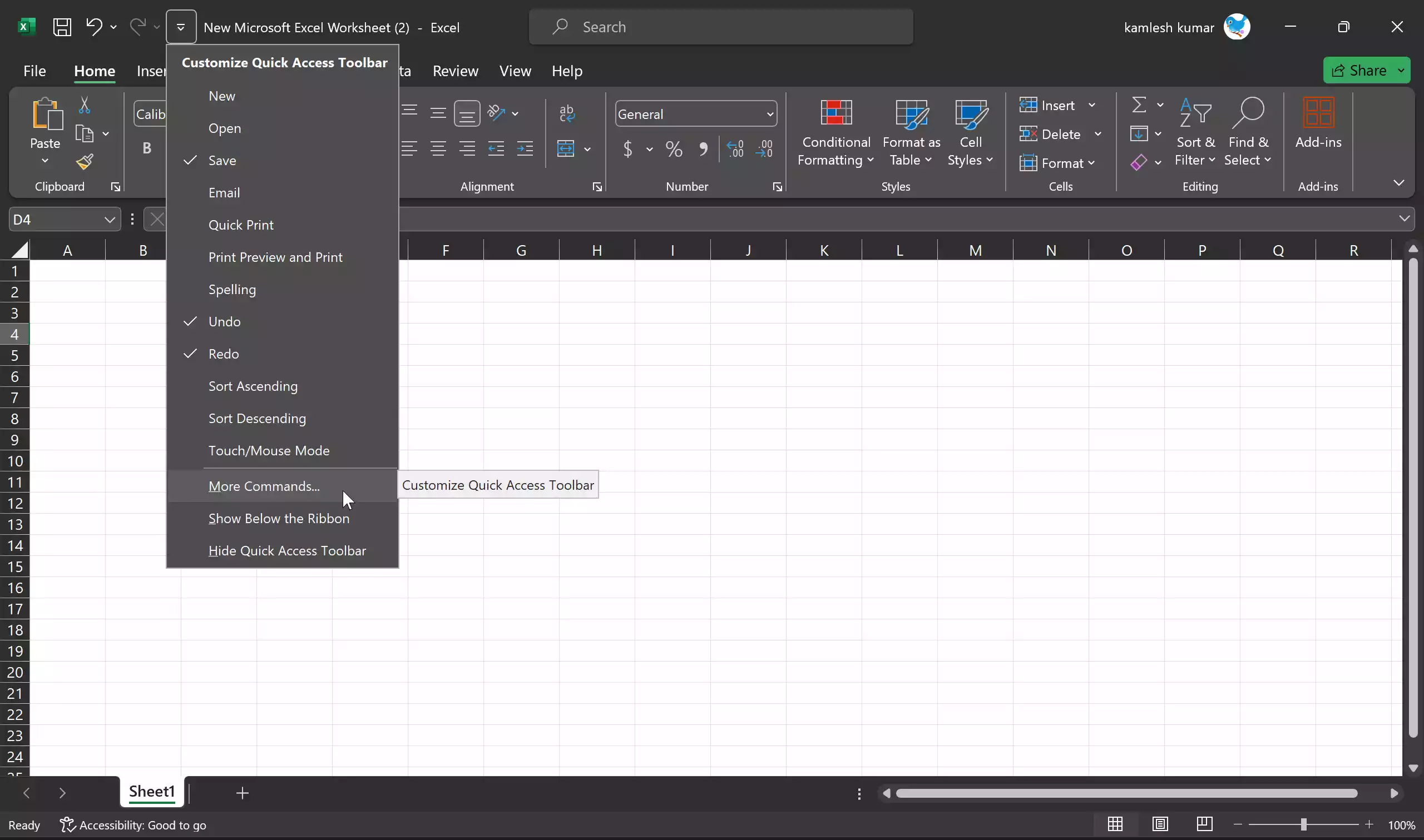
Step 3. In the dropdown menu, select “More Commands…” to open the Excel Options dialog box.
Step 4. In the Excel Options dialog box, in the “Choose commands from” dropdown menu, select “All Commands.”
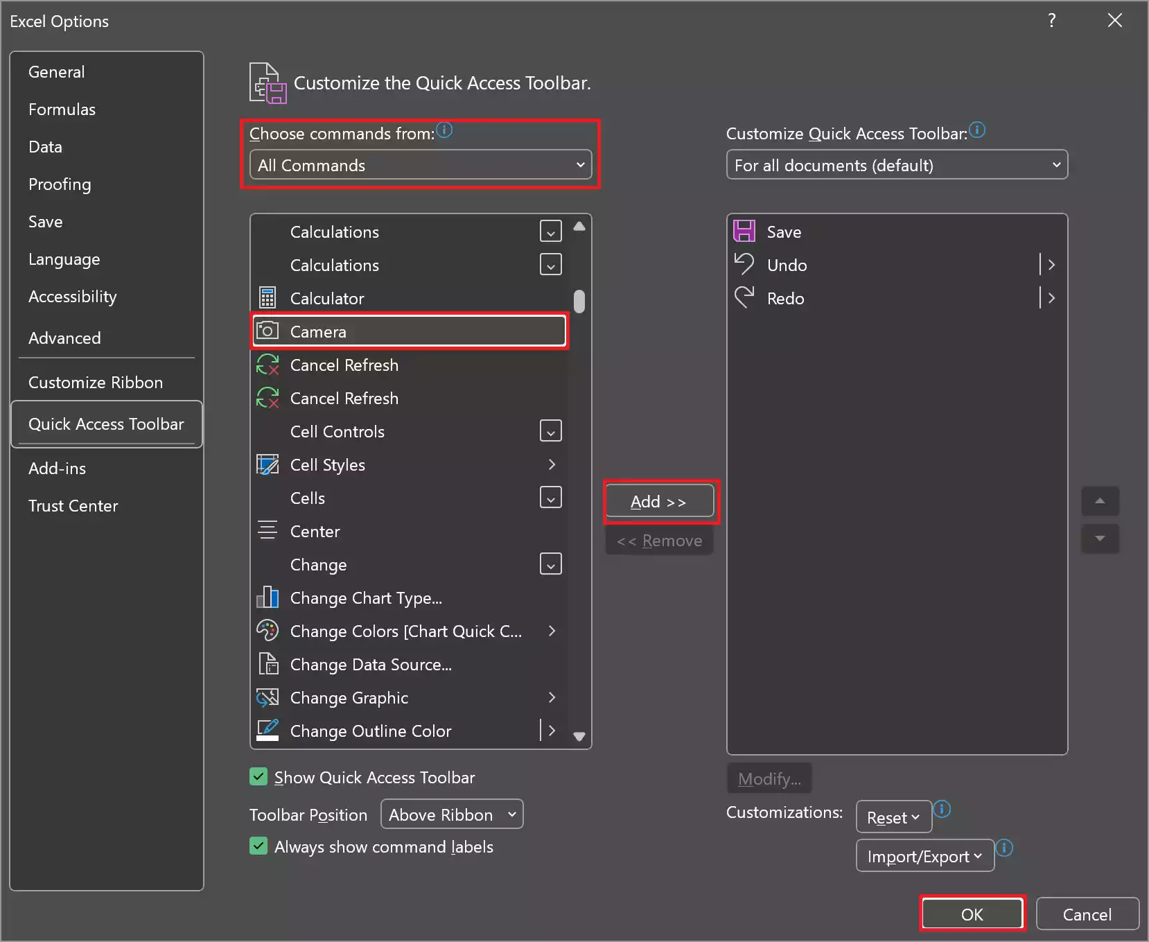
Step 5. Scroll down to find and select “Camera.”
Step 6. Click the “Add > >” button in the middle to add the Camera command to your Quick Access Toolbar.
Step 7. You can rearrange the position of the Camera command in the QAT using the “Up” and “Down” buttons on the right.
Step 8. Once you’ve added the Camera command, click “OK” to apply the changes and close the Excel Options dialog box.
With the Excel Camera added to your Quick Access Toolbar, you can now click on the Camera icon in the QAT at any time. Your cursor will turn into a crosshair. Click and drag to select the range of cells you want to capture as a snapshot. Release the mouse button, and Excel will insert a live snapshot of the selected range into your worksheet. You can move or resize the snapshot as needed.
Conclusion
Excel’s built-in screenshot tool simplifies the process of capturing and inserting screenshots directly into your spreadsheets. By following the steps outlined in this guide, you can efficiently incorporate screenshots to document your work, improve communication, and enhance presentations. Whether you’re creating reports, recording data, or illustrating your findings, Excel’s native screenshot feature is a valuable tool that can enhance your productivity and the overall quality of your Excel documents.