Microsoft Excel is a powerful tool for managing and analyzing data, but working with large spreadsheets can be a daunting task. Navigating through extensive datasets can become quite a challenge, with rows and columns seeming to stretch on forever. Fortunately, Excel provides a feature that can help make your work more efficient and organized: freezing rows and columns.
Freezing rows and columns is a technique that allows you to keep certain rows and columns visible as you scroll through your Excel spreadsheet. This is particularly useful when you have a header row or column that contains important information, such as column titles or row labels. In this gearupwindows article, we’ll explore how to freeze rows and columns in Excel, step by step.
Why Freeze Rows and Columns?
Before we dive into the “how,” let’s discuss the “why.” Freezing rows and columns in Excel has several advantages:-
Constant Reference: By freezing headers or labels, you can keep them visible as you scroll down or across your data, ensuring that you always know what each column or row represents.
Ease of Navigation: It simplifies navigation through large spreadsheets, making your work more efficient and reducing the likelihood of errors.
Data Context: You can maintain the context of your data, which is especially helpful when dealing with tables with a large number of rows and columns.
Now, let’s explore the steps to freeze rows and columns in Excel.
How to Freeze Rows in Excel?
To freeze Rows in Microsoft Excel, follow these steps:-
Step 1. Open your Excel spreadsheet that contains the data you want to work with.
Step 2. Click on the row just below the row that you want to freeze. For example, if you want to freeze the first row (containing column headers), click on the second row.
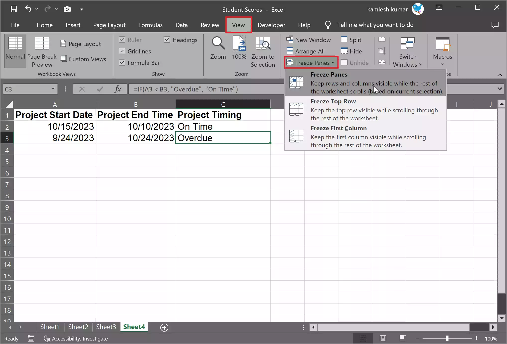
Step 3. Go to the “View” tab in the Excel ribbon.
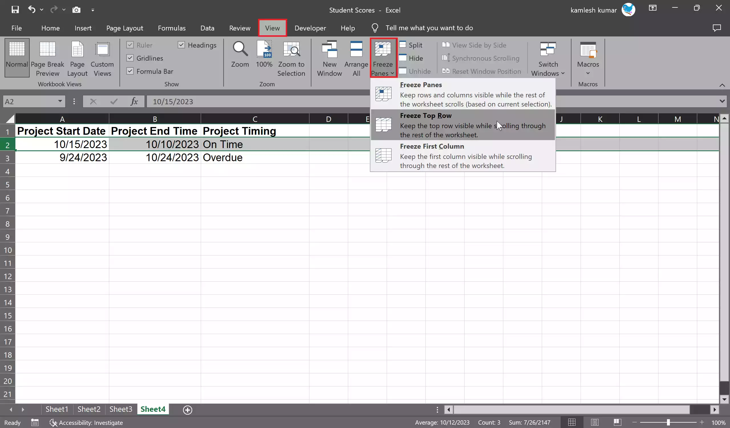
Step 4. Locate the “Freeze Panes” button in the “Window” group. Click on the drop-down arrow next to it.
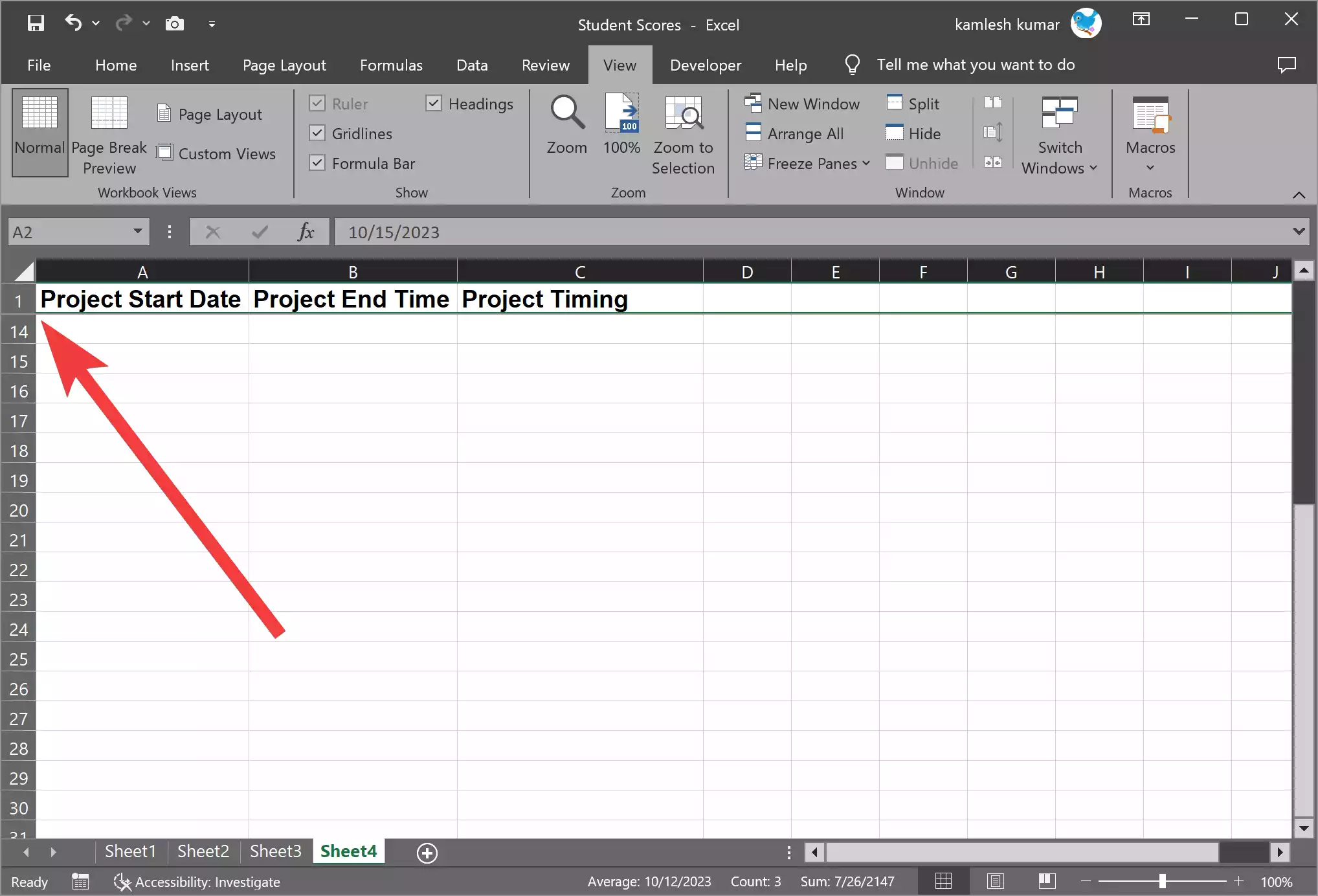
Step 5. Select “Freeze Top Row.” This will lock the top row in place. Now, when you scroll down, the top row will always be visible.
How to Freeze Columns in Excel?
To freeze Columns in Microsoft Excel, follow these steps:-
Step 1. Open your Excel spreadsheet.
Step 2. Click on the column just to the right of the column you want to freeze. For example, if you want to freeze the first column, click on the second column.
Step 3. Navigate to the “View” tab.
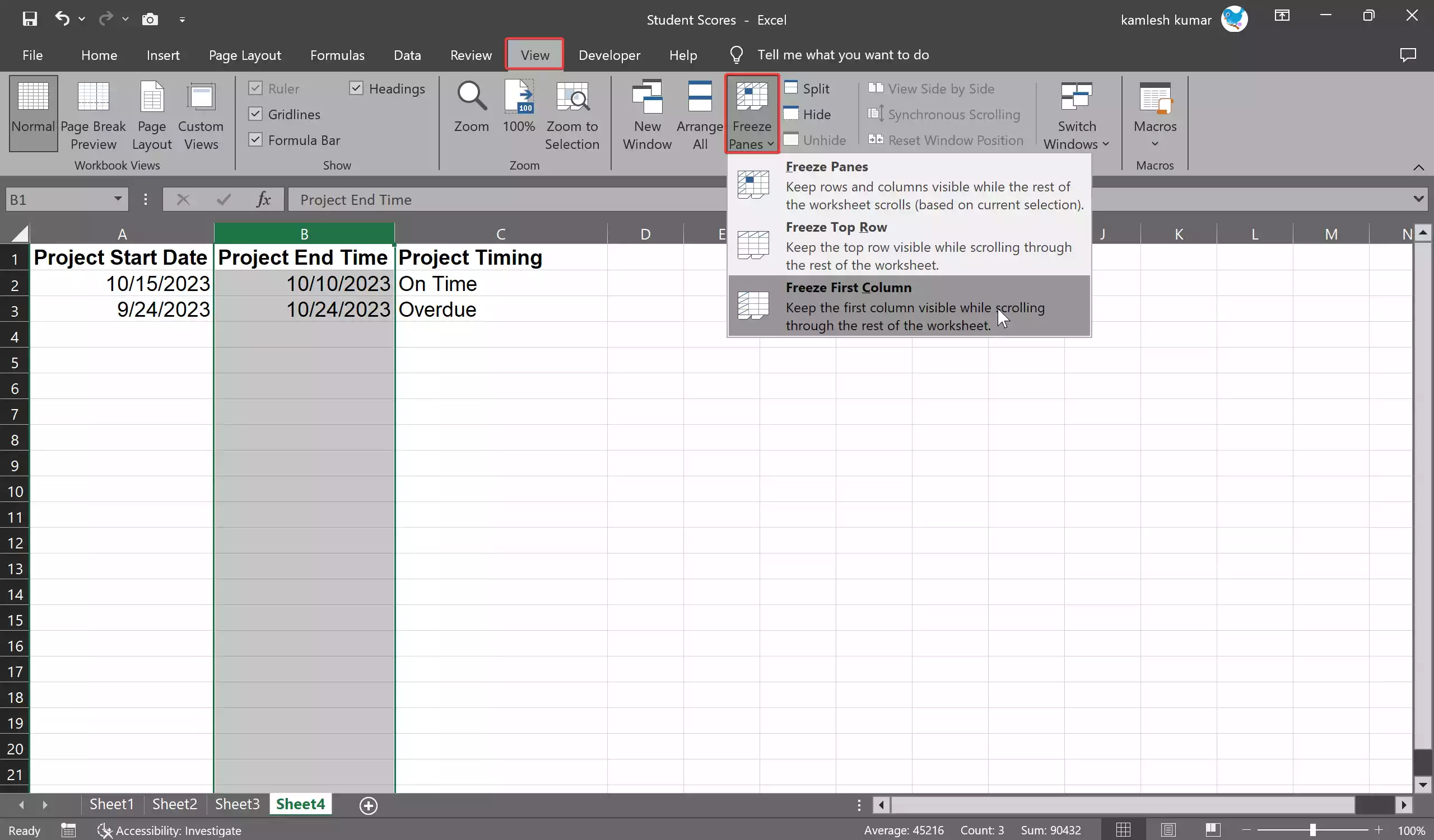
Step 4. In the “Window” group, click the “Freeze Panes” drop-down arrow.
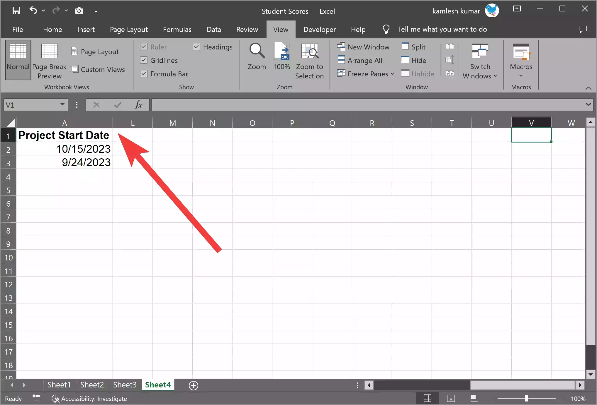
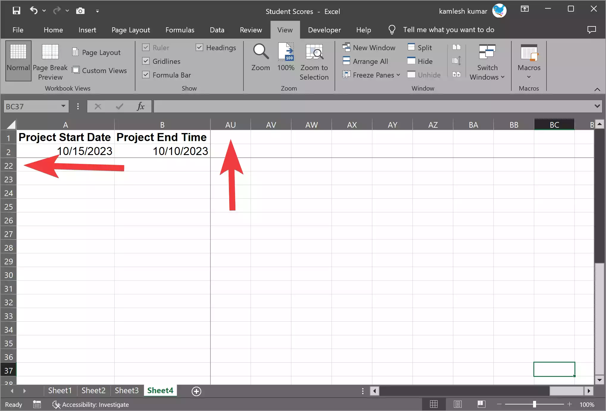
Step 5. Select “Freeze First Column.” This action locks the left column in place. When you scroll to the right, the left column will always be visible.
How to Freeze Both Rows and Columns in Excel?
Sometimes, you may need to freeze both rows and columns simultaneously. To achieve this:-
Step 1. Open your Excel spreadsheet.
Step 2. Click on the cell that is just below the last row and to the right of the last column that you want to freeze. In other words, select the cell located in the top-left corner of the area you want to keep visible.
Step 3. Go to the “View” tab.
Step 4. In the “Window” group, click the “Freeze Panes” drop-down arrow.
Step 5. Choose “Freeze Panes.” This will freeze both rows and columns to the left and above the selected cell, ensuring that your headers and labels are always in view.
How to Unfreeze Rows and Columns in Excel?
If you want to unfreeze rows or columns, follow these steps:-
Step 1. Go to the “View” tab.
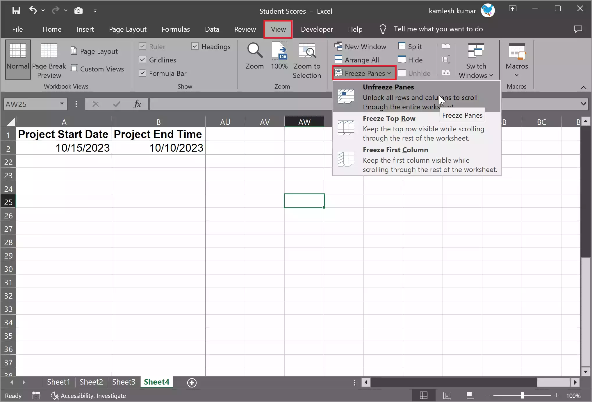
Step 2. In the “Window” group, click the “Freeze Panes” drop-down arrow.
Step 3. Select “Unfreeze Panes.”
This will remove the frozen rows and columns, allowing you to scroll through your spreadsheet freely.
Conclusion
In conclusion, knowing how to freeze rows and columns in Excel can significantly enhance your data management and analysis tasks. Whether you’re working with large datasets, complex tables, or simply want to keep your headers or labels in view, this feature is a valuable tool to make your work more efficient and less error-prone. Excel’s “Freeze Panes” option is a simple yet effective way to ensure that your essential data remains visible as you navigate through your spreadsheet.
