Microsoft Excel is a versatile spreadsheet application that offers a wide range of tools and features to help users organize and analyze data. One common task you may need to perform in Excel is hiding or unhiding rows. This can be useful for various reasons, such as focusing on specific data, making your worksheet more presentable, or concealing sensitive information. In this gearupwindows article, we’ll explore the step-by-step process for hiding and unhiding rows in Excel.
How to Hide Rows in Excel??
Hiding rows in Excel is a straightforward process. It allows you to temporarily conceal data that you don’t need to see or print but wish to keep in your worksheet for reference. Here’s how to hide rows:-
Step 1. Start by selecting the rows you want to hide. To do this, click and drag your cursor over the row numbers on the left side of the Excel window corresponding to the rows you want to hide. Alternatively, you can click on a single row number, and Excel will select that entire row. If you want to hide multiple non-contiguous rows, hold down the Ctrl key (or Command key on a Mac) while clicking on the row numbers.
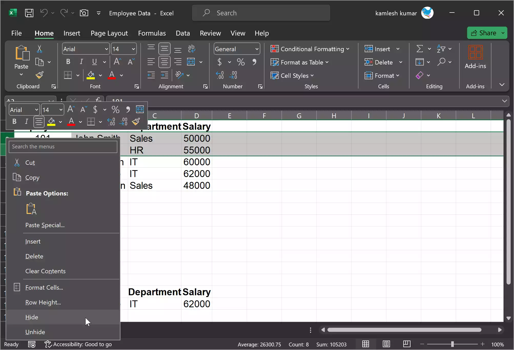
Step 2. Once you’ve selected the desired rows, right-click on any of the selected row numbers. A context menu will appear. From this menu, select “Hide.” Excel will instantly hide the selected rows, and a double line appears in the row number area, indicating hidden rows.
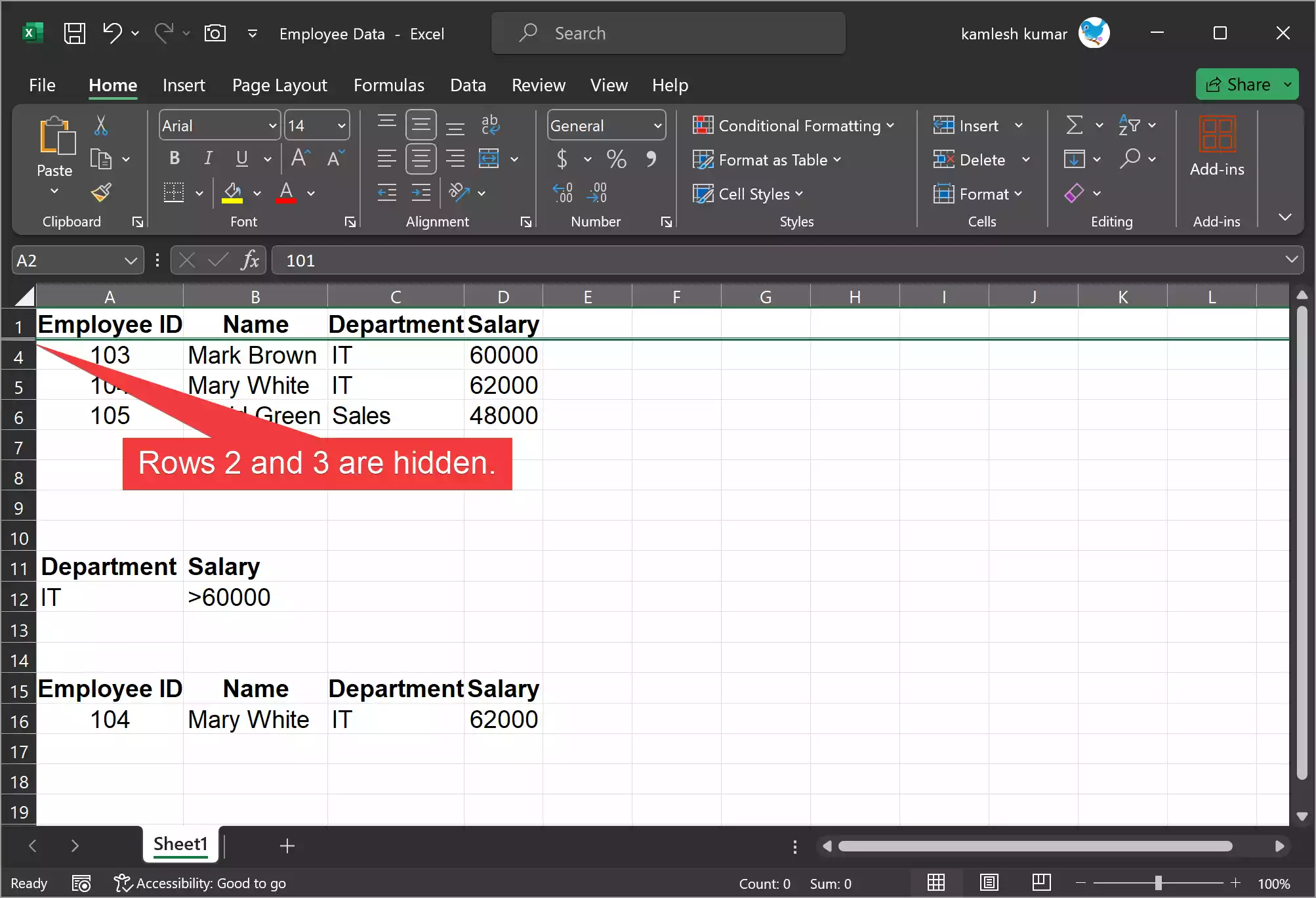
Step 3. To ensure that your rows have been hidden, look for the double line in the row number area, which is an indicator of hidden rows. You can also notice that the row numbers are no longer in consecutive order, confirming that some rows are hidden.
How to Unhide Rows in Excel??
Unhiding rows are equally simple and can be done when you want to bring back the hidden data. Here’s how to unhide rows:-
Step 1. To unhide rows, you must first select the rows above and below the hidden rows. These rows will help Excel understand where the hidden rows are located. Click and drag your cursor over the row numbers corresponding to the rows directly above and below the hidden rows.
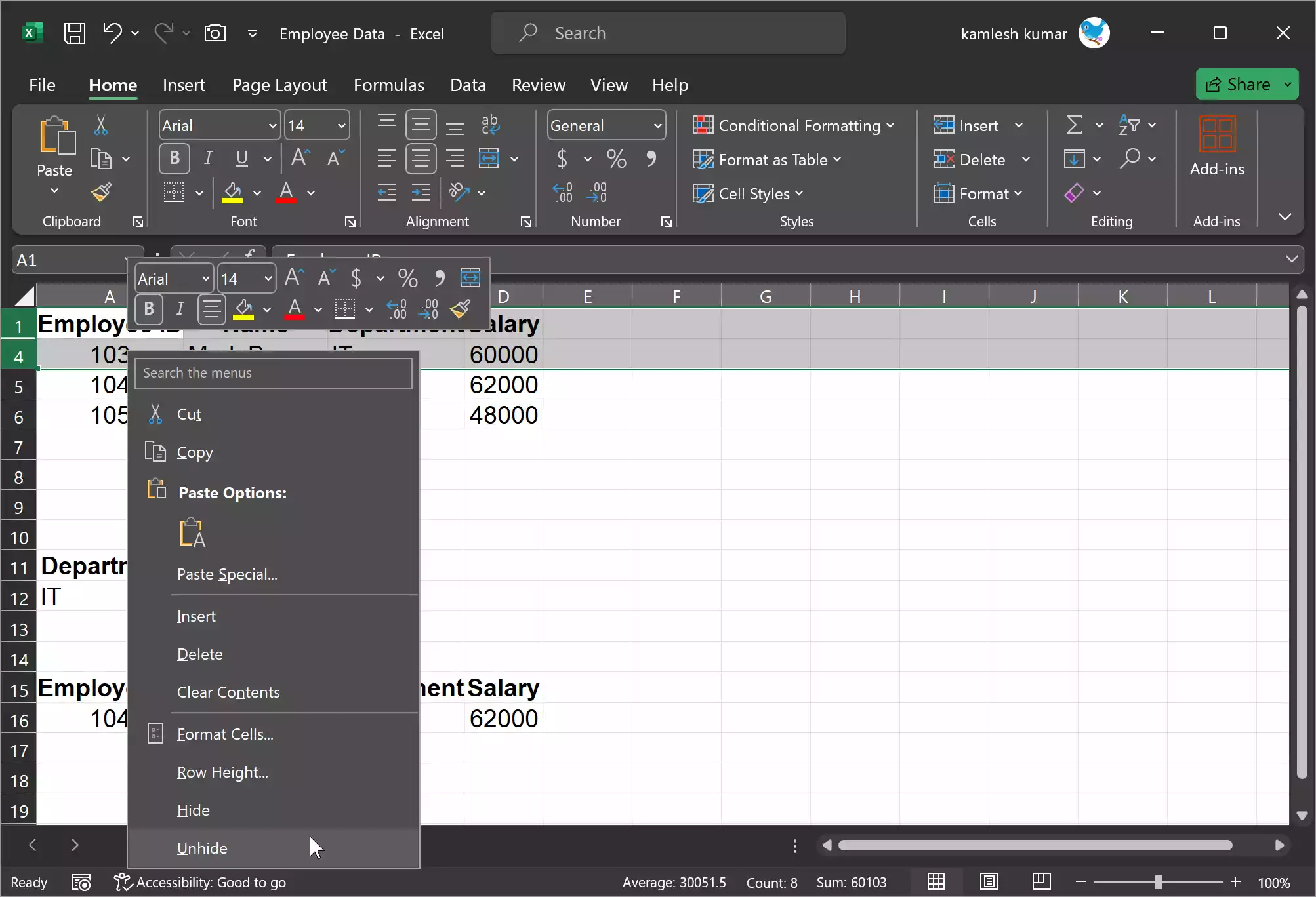
Step 2. With the adjacent rows selected, right-click on any of the selected row numbers. In the context menu that appears, choose “Unhide.” Excel will reveal the previously hidden rows.
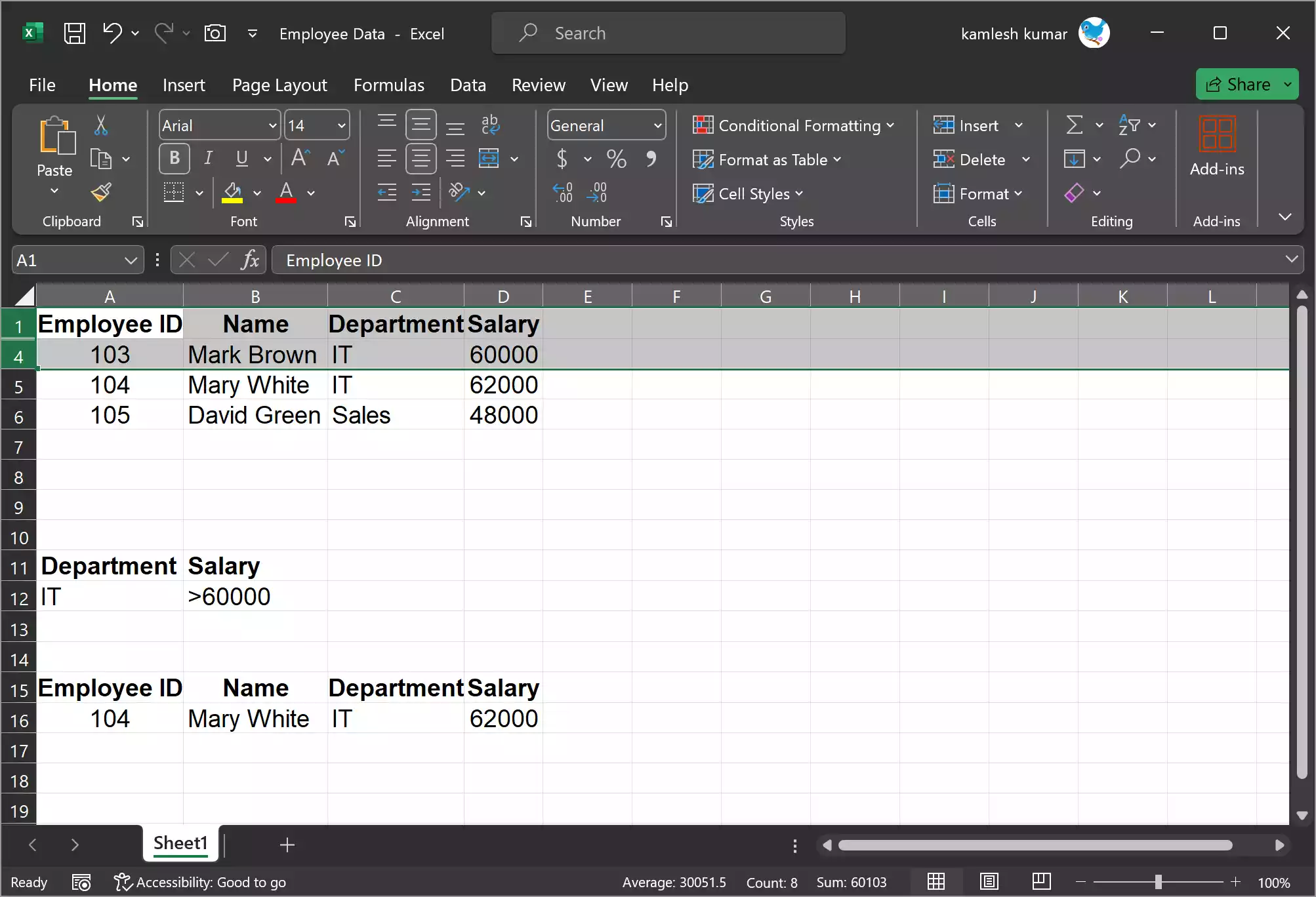
Step 3. To confirm that the hidden rows have been successfully unhidden, examine the row numbers on the left side of the Excel window. You should no longer see the double line indicator, and the row numbers will be in consecutive order again, signifying that the rows have been unhidden.
Keyboard Shortcuts for Hiding and Unhiding Rows
Excel provides keyboard shortcuts for hiding and unhiding rows, making the process even more efficient:-
– Hide Rows: Select the rows you want to hide and then press `Ctrl` + `9` (or `Cmd` + `9` on Mac). This will instantly hide the selected rows.
– Unhide Rows: To unhide rows, select the adjacent rows as described above and press `Ctrl` + `Shift` + `9` (or `Cmd` + `Shift` + `9` on Mac).
Conclusion
In summary, hiding and unhiding rows in Excel is a useful feature that can help you manage and present your data more effectively. Whether you want to focus on specific information, clean up your worksheet, or keep sensitive data out of view, Excel provides the tools to make it happen easily. By following the steps outlined in this article, you can master the art of hiding and unhiding rows in Excel and use it to your advantage in various spreadsheet tasks.
Also Read: How to Hide and Unhide Columns in Excel?