Microsoft Excel is a powerful spreadsheet program that offers a myriad of functions and features to help users organize and analyze data. One common task in Excel is linking data from one sheet to another. This allows you to create dynamic connections between different parts of your workbook, making it easier to maintain and update your data. In this gearupwindows article, we’ll explore the various methods for linking to another sheet in Excel and the practical applications of this feature.
Why Link to Another Sheet?
Linking to another sheet is a valuable technique in Excel for several reasons:-
1. Data Organization: It helps organize your data, especially in complex workbooks with multiple sheets. You can keep related information on separate sheets while maintaining easy access to all relevant data.
2. Data Consistency: Linked data stays consistent and up-to-date. When you change data in one sheet, the linked data in another sheet is automatically updated. This minimizes the risk of errors resulting from manual data entry.
3. Data Presentation: Linking allows you to create summary sheets that display critical information from multiple other sheets. This is useful for creating dashboards or reports.
4. Data Analysis: Linked data can be used in calculations, charts, and graphs, making it easier to perform various analyses on your data.
Now, let’s explore different methods for linking to another sheet in Excel.
How to Link to Another Sheet in Microsoft Excel?
Method 1: Simple Cell Reference
The most straightforward way to link to another sheet is to use cell references. To do this, follow these steps:-
Step 1. In the cell where you want to display linked data, type an equal sign (=).
Step 2. Click on the sheet where the data is located (the sheet name appears at the bottom of the Excel window).
Step 3. Click on the cell containing the data you want to link to.
Step 4. Press Enter.
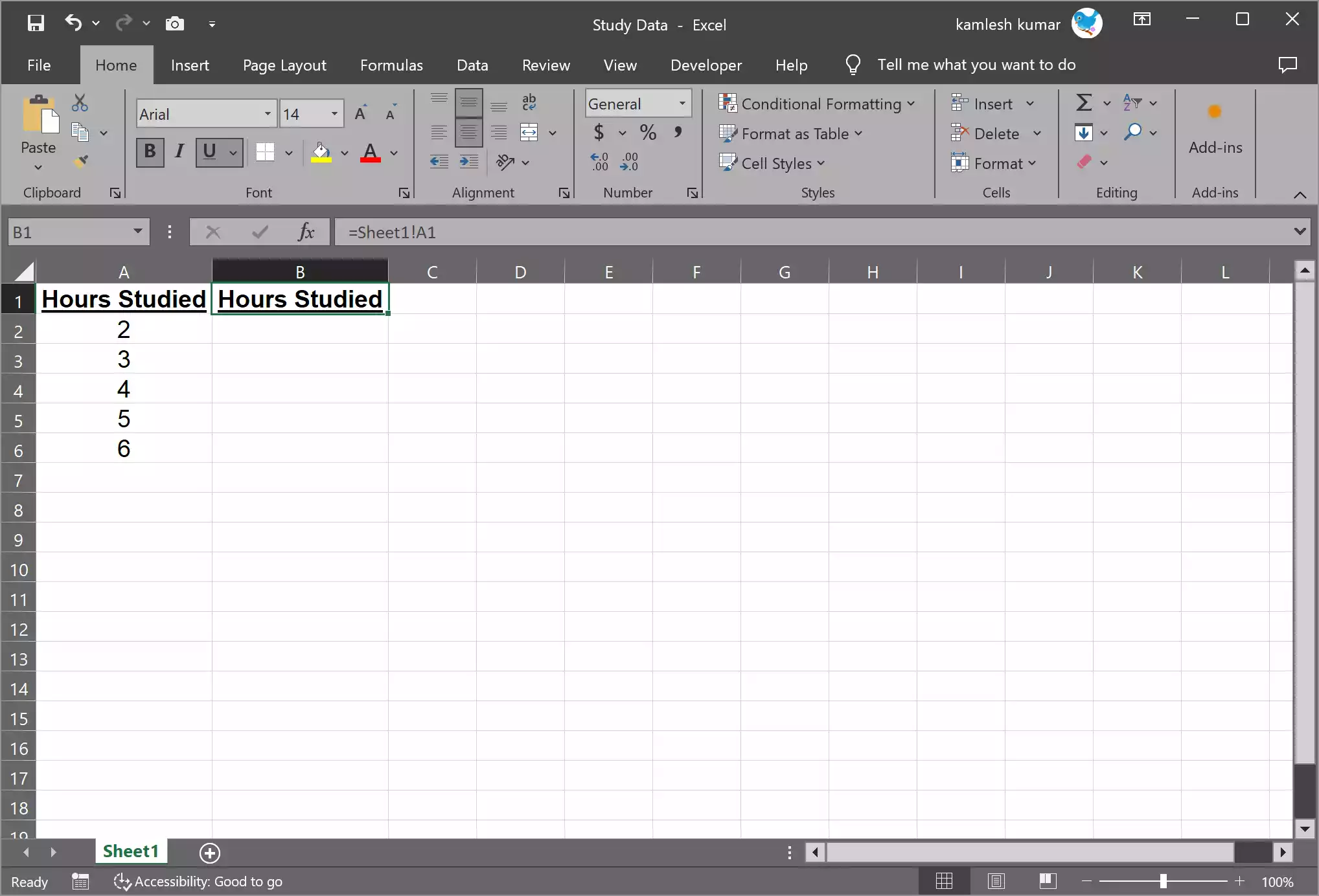
For example, if you have data in cell A1 on a sheet named “Sheet1,” and you want to link it to cell B1 on your current sheet, you would enter the formula `=Sheet1!A1` in cell B1.
Method 2: Using Named Ranges
Named ranges are a great way to create dynamic links between sheets. You can define a name for a range of cells and then use that name in formulas. This method is particularly useful when working with large data sets or complex workbooks.
To use named ranges:-
Step 1. Select the range of cells you want to name.
Step 2. Go to the “Formulas” tab and click on “Define Name.”
Step 3. Enter a name for the range.
Step 4. Click “OK.”
Now, you can use this name in your formulas to link to another sheet. For example, if you named a range “SalesData” that includes data in “Sheet1,” you can link to it using the formula `=SalesData.`
Method 3: 3D Reference
When you have data spread across multiple sheets with the same layout, you can use a 3D reference to consolidate it. This method allows you to perform calculations or create summaries across multiple sheets.
Here’s how to use a 3D reference:-
Step 1. In the cell where you want to display the linked data, type an equal sign (=).
Step 2. Select the range of cells you want to reference, but do not include the sheet name.
Step 3. After selecting the range, add the sheet names and exclamation points for the sheets you want to reference. For example, to reference cell A1 on “Sheet1” and “Sheet2,” you would enter `=’Sheet1:Sheet2′!A1.
Step 4. Press Enter.
This method is particularly handy when you have many sheets with the same structure, such as monthly sales reports.
Assuming you have sales data in cells B2 to B5 in sheets “Q1,” “Q2,” “Q3,” and “Q4,” and you want to calculate the sum of those values in the “Summary” sheet, you can use the `SUM` function with a 3D reference. Here’s how to do it:-
Step 1. In the “Summary” sheet, select the cell where you want to display the total sales.
Step 2. Enter the following formula:-
=SUM('Q1:Q4'!B2:B5)
Step 3. Press Enter.
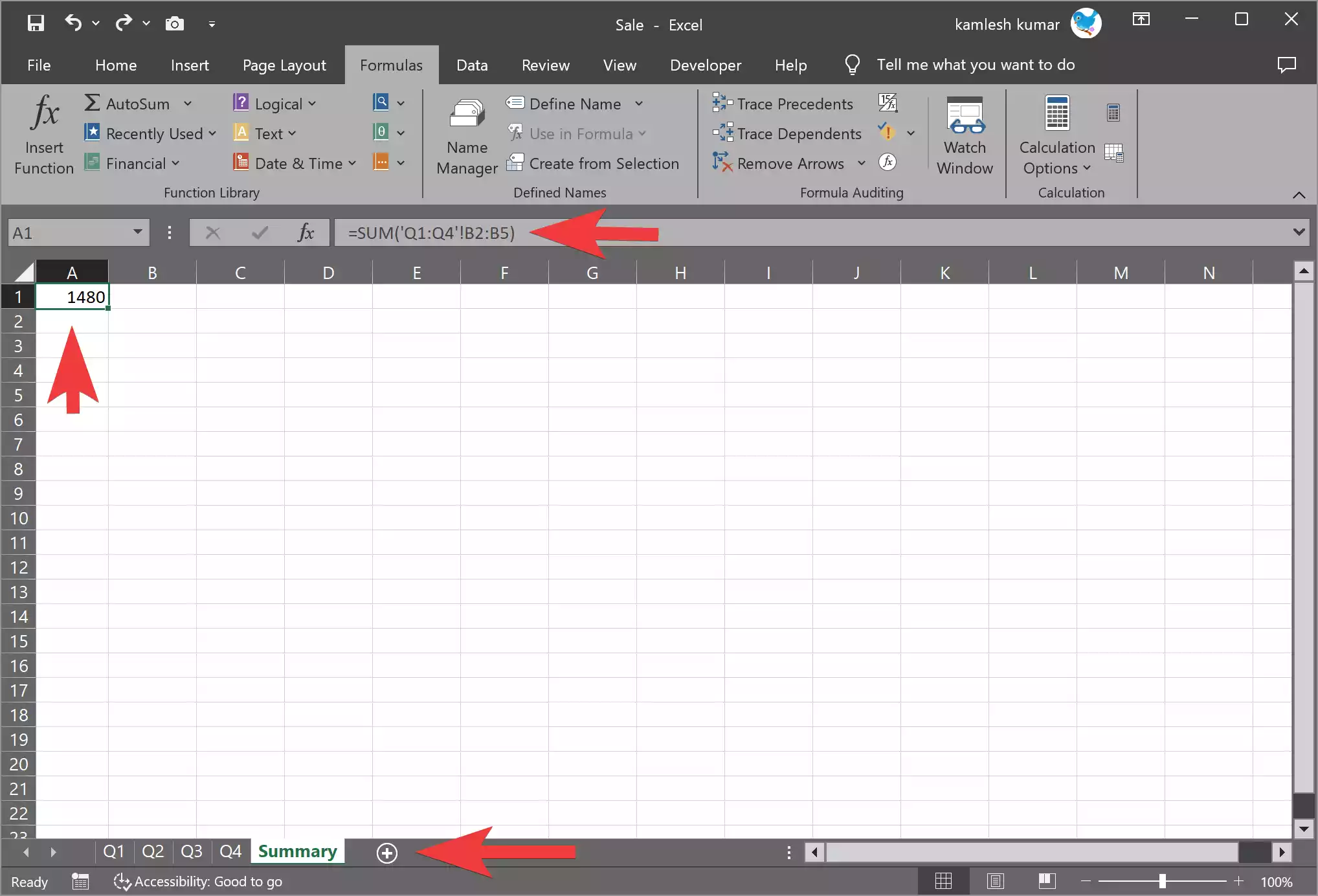
Make sure to include single quotation marks around the sheet names (e.g., ‘Q1:Q4’) within the formula.
Now, Excel should correctly calculate the sum of the values in cells B2 to B5 from the “Q1” to “Q4” sheets and display the total in the “Summary” sheet.
Method 4: Hyperlinking
Another way to link to another sheet is by using hyperlinks. This method is useful when you want to create easy navigation within your workbook. Here’s how to do it:-
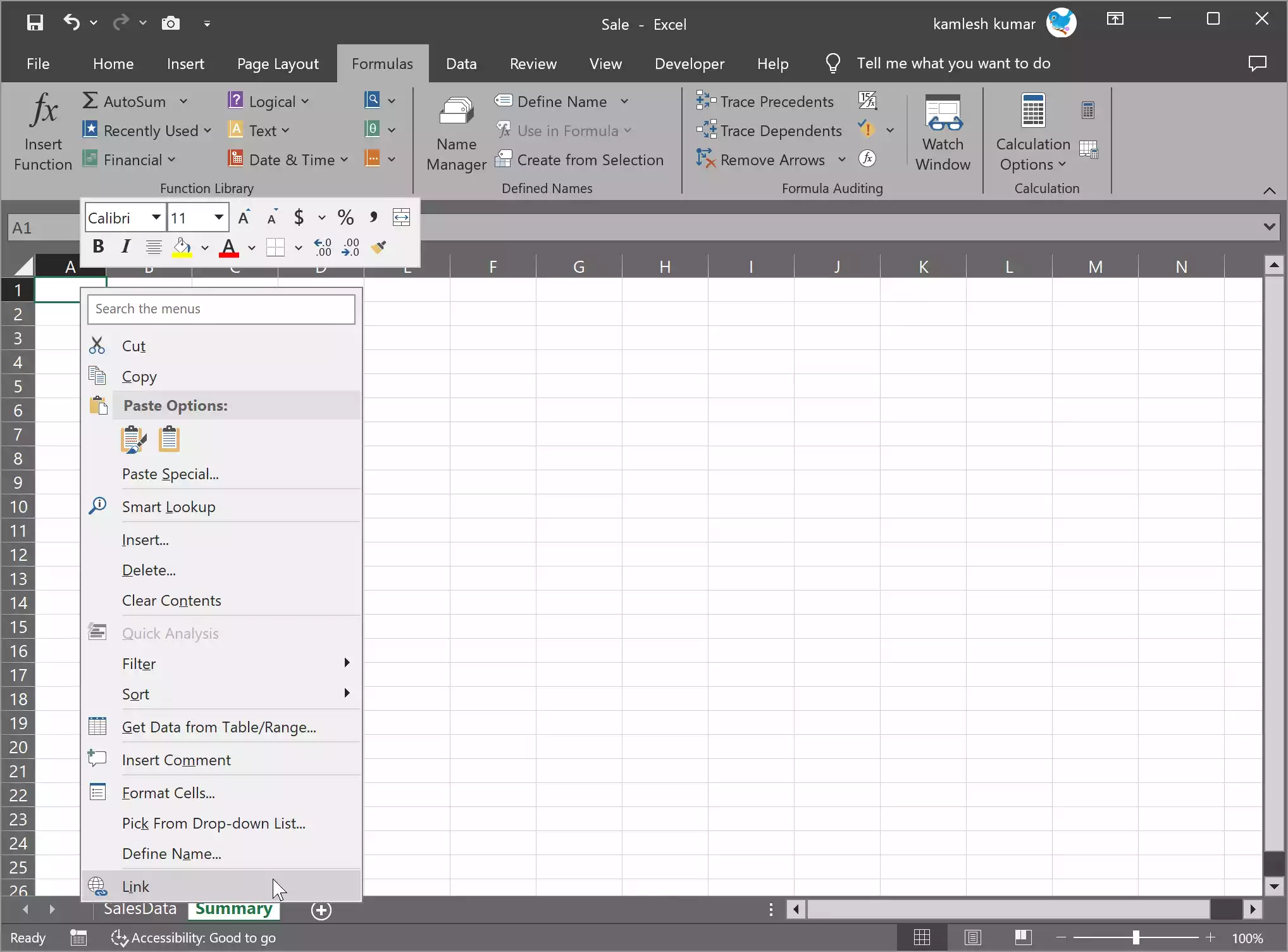
Step 1. Select the cell or text that you want to turn into a hyperlink.
Step 2. Right-click and choose “Hyperlink” from the context menu.
Step 3. In the “Insert Hyperlink” dialog box, select “Place in This Document.”
Step 4. Choose the sheet you want to link to from the list.
Step 5. Select the specific cell reference, if needed.
Step 6. Click “OK.”
Now, clicking on the hyperlink will take you to the linked sheet.
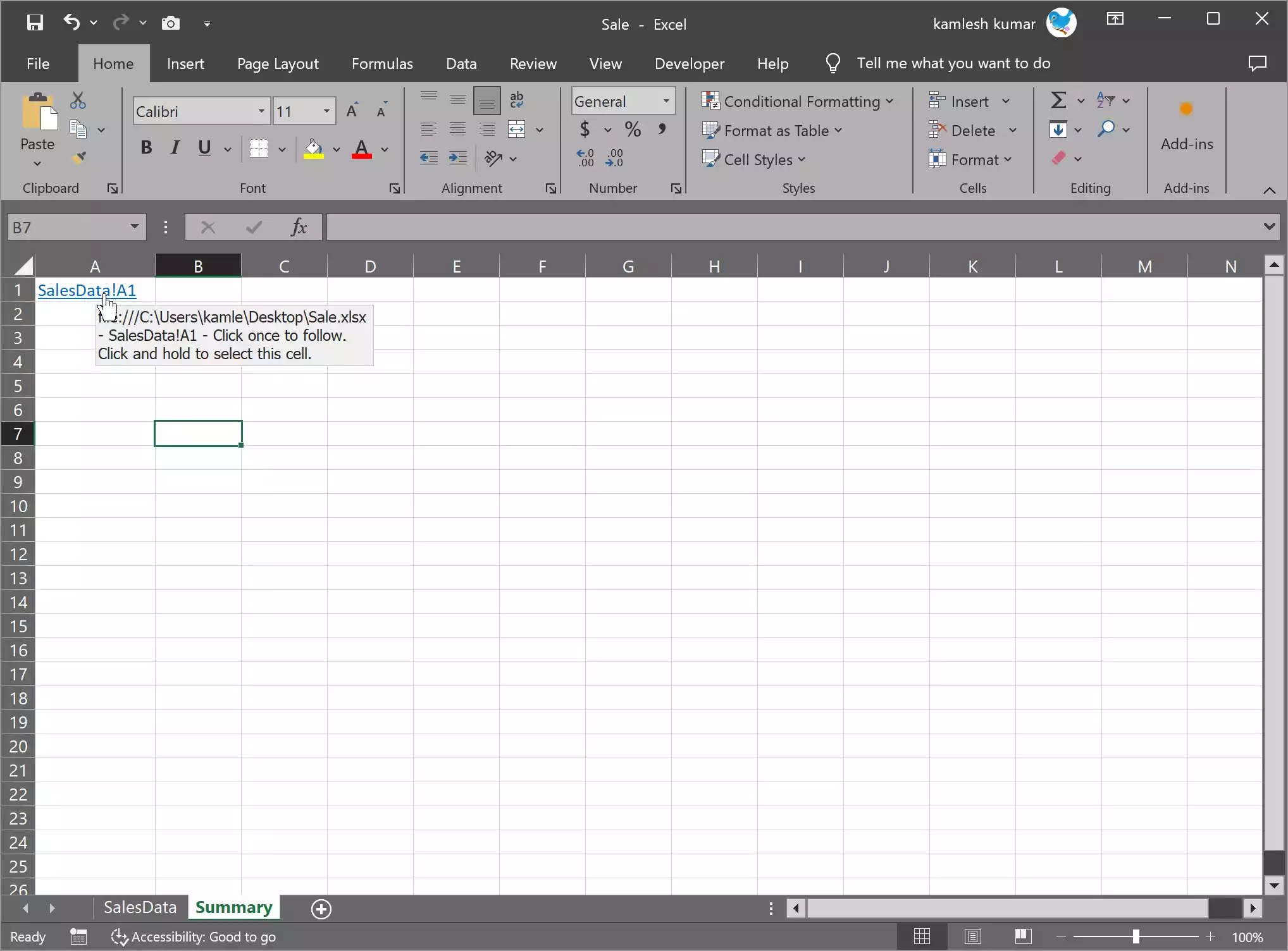
Let’s say you have an Excel workbook with two sheets: “SalesData” and “Summary.” You want to create a hyperlink in the “Summary” sheet that allows you to quickly jump to the “SalesData” sheet.
Follow these steps:-
Step 1. Open your Excel workbook with the two sheets (“SalesData” and “Summary”).
Step 2. In the “Summary” sheet, select the cell where you want to create the hyperlink. Let’s say you want to link it from cell A1.
Step 3. Right-click on cell A1 and choose “Link” or “Hyperlink” from the context menu. This will open the “Insert Hyperlink” dialog box.
Step 4. In the “Insert Hyperlink” dialog box, in the “Link to” section, select “Place in This Document.”
Step 5. In the “Or select a place in this document” section, you will see a list of all the sheets in your workbook. Click on “SalesData” to select it. Optionally, you can specify a cell reference within the “SalesData” sheet. For example, if you want to link to cell A1 in “SalesData,” type “A1” in the “Type the cell reference” field.
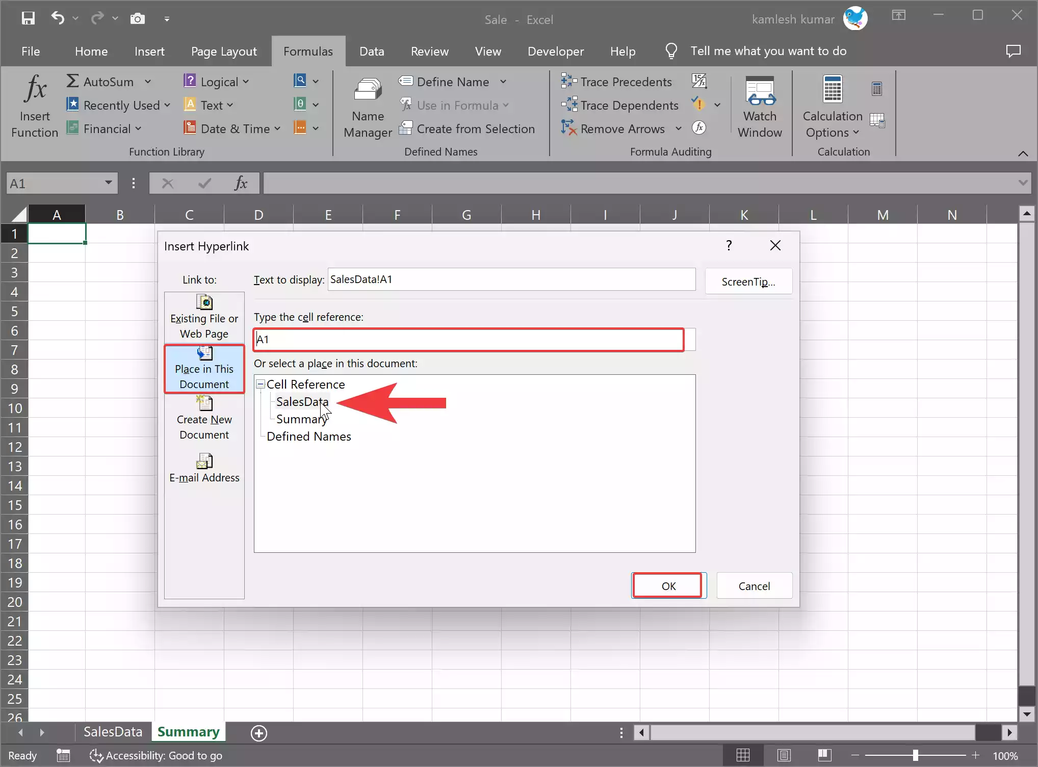
Step 6. After selecting the sheet and (if needed) the cell reference, click “OK” to create the hyperlink.
Now, when you click on the cell in the “Summary” sheet (cell A1 in this case), it will act as a hyperlink, and clicking it will take you directly to the “SalesData” sheet or the specified cell within it.
This hyperlink is a convenient way to navigate within your Excel workbook, especially when you have a large number of sheets and want to create a table of contents or summary sheet that provides quick access to other sections of your workbook.
Practical Applications
The ability to link to another sheet in Excel has numerous practical applications:-
1. Financial Modeling: In financial models, you can link various components of the income statement, balance sheet, and cash flow statement to create dynamic and interconnected financial models.
2. Project Management: When managing a project, you can link task lists and timelines across multiple sheets, providing an overview on a master sheet while maintaining detailed information on individual sheets.
3. Inventory Management: Linking inventory data across different locations or categories simplifies inventory tracking and analysis.
4. Sales Reports: You can create dynamic sales reports by linking data from different months or quarters into a summary sheet.
5. Dashboard Creation: Excel dashboards often rely on linked data to display key performance indicators (KPIs) from various sources.
Conclusion
In conclusion, linking to another sheet in Excel is a fundamental skill that can greatly enhance the functionality and organization of your workbooks. Whether you’re a data analyst, a financial modeler, or a project manager, mastering these techniques will help you efficiently manage and analyze data while reducing the risk of errors. With these methods in your Excel toolkit, you can take your spreadsheet skills to the next level.
