Microsoft Excel is a versatile and powerful spreadsheet software that is widely used in business, finance, and various other fields. One of its essential features is the ability to work with date and time data. Whether you’re tracking project deadlines, managing schedules, or analyzing trends, mastering date and time functions in Excel is crucial. In this gearupwindows article, we will explore various date and time functions in Excel and provide a step-by-step guide on how to use them effectively.
Understanding Date and Time Formats
Before delving into the specific functions, it’s important to understand how Excel handles date and time data. Excel stores dates as serial numbers, with each date corresponding to a unique number. Time is represented as a fraction of a day. This system makes it easy to perform calculations and manipulate date and time data within Excel.
Common Date and Time Functions
Excel offers a wide range of functions to work with date and time data. Here are some of the most commonly used functions:-
TODAY() and NOW()
– `TODAY()` returns the current date.
– `NOW()` returns the current date and time.

These functions are often used to update cells with the current date or time automatically.
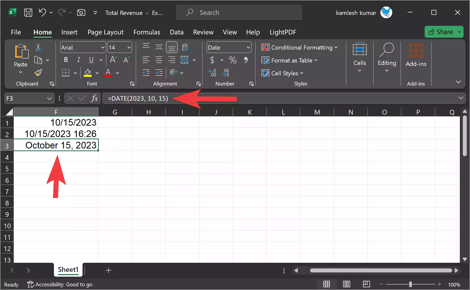
DATE(year, month, day)
This function allows you to create a date by specifying the year, month, and day as arguments. For example, `=DATE(2023, 10, 15)` would return October 15, 2023.
TIME(hour, minute, second)
Similarly, you can create a specific time using the `TIME()` function. It takes the hour, minute, and second as arguments. For example, `=TIME(14, 30, 0)` would return 2:30 PM.

DATEDIF(start_date, end_date, unit)
The `DATEDIF()` function calculates the difference between two dates in various time units (days, months, or years). For example, `=DATEDIF(A1, A2, “d”)` calculates the number of days between the dates in cells A1 and A2.

YEAR(), MONTH(), DAY()
These functions allow you to extract the year, month, or day from a date. For instance, `=YEAR(A1)` will return the year of the date in cell A1. Similarly, you can use =MONTH(A1) to return the month of the date in cell A1 and =DAY(A1) to return the day of the month.

HOUR(), MINUTE(), SECOND()
Similarly, you can extract the hour, minute, or second from a time using these functions.
EOMONTH(start_date, months)
The `EOMONTH()` function returns the last day of a month after adding or subtracting a specified number of months from the given start date. It’s particularly useful for financial and billing calculations.
Suppose you want to calculate the end date of a project that starts on January 10, 2023, and is expected to last for 6 months. You want to find the last day of the month that is six months after the project start date.
Here’s how you can use the `EOMONTH()` function for this calculation:-
In an Excel spreadsheet, enter your start date in cell A1. In this case, you would enter “01/10/2024.” In cell B1, enter the number of months the project will last. In this example, you would enter “6.” Then, in a cell where you want to display the end date, enter the following formula:-
=EOMONTH(A1, B1)

This formula calculates the last day of the month after adding the number of months specified in cell B1 to the start date in cell A1.
After entering the formula, press Enter, and Excel will calculate the result.
To make the result more readable, format the cell to display the date in a preferred format. Right-click the cell with the result, choose “Format Cells,” and select a date format that you like.
The cell containing the `EOMONTH()` formula will now display the last day of the month that is six months after the project start date.
In this example, if cell A1 contains “01/10/2024” (January 10, 2024), and cell B1 contains “6” (indicating 6 months), the formula will return “07/31/2024” (July 31, 2024) as the end date, which is the last day of the month that is six months after the project start date.
You can modify the start date and the number of months in cells A1 and B1 to perform similar calculations for different scenarios. Excel’s `EOMONTH()` function is a valuable tool for handling various date-related calculations, especially in financial and scheduling contexts.
NETWORKDAYS(start_date, end_date, [holidays])
This function calculates the number of working days (weekdays) between two dates, excluding specified holidays. You can include a list of holidays as an optional argument.
Suppose you’re tasked with calculating the number of working days between two dates, and you also want to exclude specific holidays. Here’s how you can use the `NETWORKDAYS()` function:-
First, enter your date data into Excel. In cell A1, enter the start date, and in cell A2, enter the end date. In cells A3 and below, list the holidays you want to exclude, if any.
For this example, let’s say you have the following data:
- Start Date (A1): 2024-10-01 (October 1, 2024)
- End Date (A2): 2024-10-10 (October 10, 2024)
- Holidays (A3 and A4): 2024-10-03 (October 3, 2024) and 2024-10-02 (October 2, 2024)
In a cell where you want to display the number of working days, you can use the `NETWORKDAYS()` function. Let’s assume you want the result in cell B1. Enter the following formula:-
=NETWORKDAYS(A1, A2, A3:A4)
In this formula:-
- `A1` is the start date.
- `A2` is the end date.
- `A3:A4` is the range of cells containing the holidays.
Note: The NETWORKDAYS() function in Excel does not automatically exclude weekends (Saturdays and Sundays) by default. However, you can easily modify the function to exclude weekends as well by customizing it to suit your needs. To exclude weekends (Saturdays and Sundays) in addition to specific holidays, you can modify the function like this:-
=NETWORKDAYS(A1, A2, A3:A4, 1, 1)
When you’re done, press Enter, and Excel will calculate the number of working days between the start date and end date, excluding the specified holidays.

The result will appear in cell B1, which, in this example, would be “6” because there are 6 working days between October 1, 2024, and October 10, 2024, excluding the holidays on October 3, 2024, and October 2, 2024.
You can adjust the start date, end date, and holidays as needed to calculate working days for different date ranges and sets of holidays. This function is especially useful for project planning, leave tracking and other scenarios where you need to determine the number of working days within a specific period while considering holidays.
NOW()
The `NOW()` function returns the current date and time, and it’s commonly used for real-time tracking or time-sensitive calculations.
Applying Date and Time Functions
To apply these functions effectively, follow these steps:-
Step 1. Enter Date and Time Data: Start by entering your date and time data into Excel. Ensure that the cells are correctly formatted as dates or times to prevent any errors.
Step 2. Select the Cell for the Result: Choose the cell where you want to display the result of your date or time function.
Step 3. Enter the Function: Type the desired function in the selected cell, following the function’s syntax and arguments. For example, to calculate the difference between two dates, you would type `=DATEDIF(A1, A2, “d”)` in the cell.
Step 4. Press Enter: After entering the function, press Enter, and Excel will calculate and display the result.
Step 5. Format the Result: To make the result more readable, you can format the cell containing the function result. Right-click the cell, choose Format Cells, and select a date or time format that suits your needs.
Tips for Working with Date and Time Functions
Here are some additional tips to help you master date and time functions in Excel:-
Step 1. Be Consistent: Ensure that your date and time data is consistent and properly formatted throughout your spreadsheet. This prevents calculation errors.
Step 2. Use Absolute References: When working with functions that reference other cells, consider using absolute references (e.g., $A$1) to lock the cell references. This prevents them from changing when you copy or drag the formula to other cells.
Step 3. Include Error Handling: Date and time functions can result in errors, especially if the input data is inconsistent. Use error handling functions like `IFERROR()` to display custom messages or values when errors occur.
Step 4. Use Named Ranges: For complex worksheets with many date and time calculations, consider defining named ranges for your date and time data. This makes your formulas more readable and maintainable.
Step 5. Practice and Experiment: The best way to master date and time functions in Excel is to practice and experiment with different functions and scenarios. Excel provides a variety of tools for working with date and time, so explore and familiarize yourself with these functions.
Conclusion
In conclusion, mastering date and time functions in Excel is essential for efficiently managing and analyzing data. Whether you are tracking deadlines, creating schedules, or conducting financial analysis, Excel’s date and time functions can greatly simplify your tasks. With the knowledge and tips provided in this article, you can become proficient in using these functions to your advantage, ultimately saving time and improving the accuracy of your work.
