Microsoft Excel is a powerful spreadsheet software that offers a wide range of functions and features to help users manipulate and analyze data effectively. One such function is the OFFSET function, which allows you to dynamically reference a range of cells based on a specified starting point. This function can be particularly useful for creating dynamic reports, dashboards, and charts. In this article, we’ll explore the OFFSET function in detail and provide examples of its usage.
Syntax of the OFFSET Function
Before delving into examples, it’s essential to understand the syntax of the OFFSET function:-
=OFFSET(reference, rows, columns, [height], [width])
– reference: This is the starting point or reference cell from which you want to offset. It’s usually a cell or a range of cells.
– rows: This argument determines the number of rows to move vertically from the reference cell. A positive number means moving down, while a negative number means moving up.
– columns: This argument specifies the number of columns to move horizontally from the reference cell. A positive number indicates moving right, while a negative number indicates moving left.
– [height] (optional): This argument is used to define the height or the number of rows in the resulting range. If omitted, Excel will default to a single cell.
– [width] (optional): This argument defines the width or the number of columns in the resulting range. If omitted, Excel will default to a single cell.
How to Use the Excel OFFSET Function?
Basic Offset Function Example
Suppose you have the following data in cells A1 to A5:-

Now, you want to use the OFFSET function to retrieve the value in cell A3 (which is “Cherry“). You can use the formula:-
=OFFSET(A1, 2, 0)
Here, `A1` is the reference cell, `2` represents moving 2 rows down, and `0` signifies no horizontal movement. The result will be “Cherry.”
Dynamic Range Example
You have a sales data table with the following structure:-
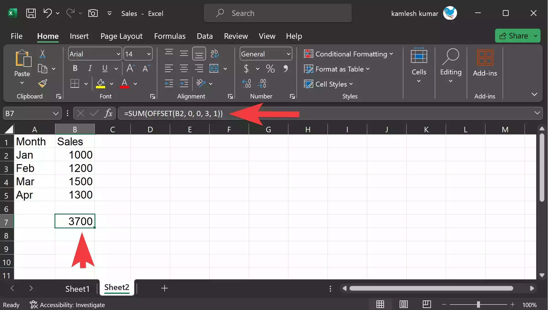
=SUM(OFFSET(B2, 0, 0, 3, 1))
If you want to create a dynamic sum of the sales for the first three months, you can use the OFFSET function in combination with the SUM function:-
=SUM(OFFSET(B2, 0, 1, 3, 1))
Here, `B2` is the reference cell, `0` rows to move (no vertical movement), `1` column to move (no horizontal movement), `3` rows high (represents the range from Jan to Mar), and `1` column wide (indicating the “Sales” column). The result will be the sum of the sales for Jan, Feb, and Mar, which is `3700`.
Important Tips and Considerations
- The OFFSET function can be volatile, meaning it recalculates every time there is any change in the worksheet. Overuse of OFFSET can slow down your Excel workbook, especially in large datasets. In such cases, consider using alternative functions like INDEX and MATCH or dynamic named ranges.
- Be cautious when using OFFSET with extremely large ranges, as it can significantly impact performance.
- Always ensure that the row and column offsets you provide are within the boundaries of your data to avoid errors.
Conclusion
In conclusion, the Excel OFFSET function is a powerful tool for creating dynamic spreadsheets and charts. By understanding its syntax and examples, you can harness its capabilities to build interactive and responsive worksheets that adapt to changes in your data.
