One of the most popular spreadsheet applications is Excel, which is widely used across a wide range of industries. However, it has a special place in the business and accounting fields because it has many built-in accounting-friendly features that make it very easy to use. One of these features is the Accounting Number Format, which Excel uses when working with money-related data.
Using Excel, you can create financial reports, analyze data, and more. Many accountants use Excel to store, organize, and analyze financial data. It is important to maintain consistent formatting across cells when working with financial values. Using accounting number format in your workbooks can help you format your values consistently, making them easier to use and review.
There are multiple ways to apply accounting number formatting to your numbers if you use Microsoft Excel for accounting purposes. Here’s how.
This gearupwindows article will show you how to apply accounting number format in Excel, and if you are looking for how to apply accounting number format, then you’ve come to the right place.
What is Accounting Number Format?
Similar to the Currency format, Accounting Number Format can be applied to numbers as needed. The accounting format differs from the currency format, such as:-
Accounting Number Format displays the currency sign in a column to the left of the cell, whereas Currency Format shows the currency sign next to the number.
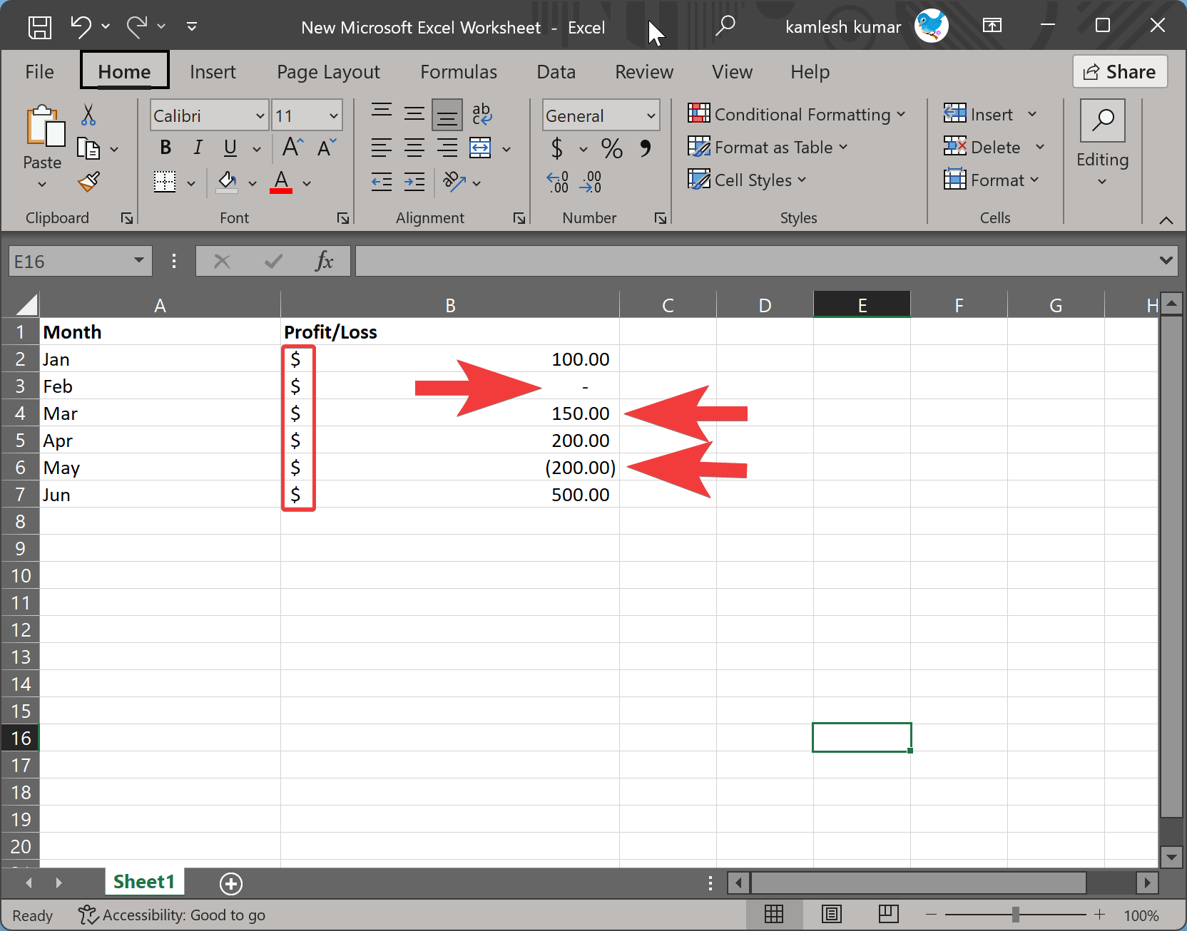
Zero values display as ‘–’ (dash) in Accounting Number Format, but Currency Format displays it as 0.
Negative numbers display in parentheses () in Accounting Number Format, however, Currency Format displays negative numbers with a ‘–’ (minus) symbol.
Note: The Excel program does not display negative numbers in parenthesis by default. It is an optional setting that accountants can set.
How to Apply the Accounting Number Format in Excel using the Accounting Number Format icon?
To use the accounting number format in Excel through the Accounting Number Format icon, use these steps:-
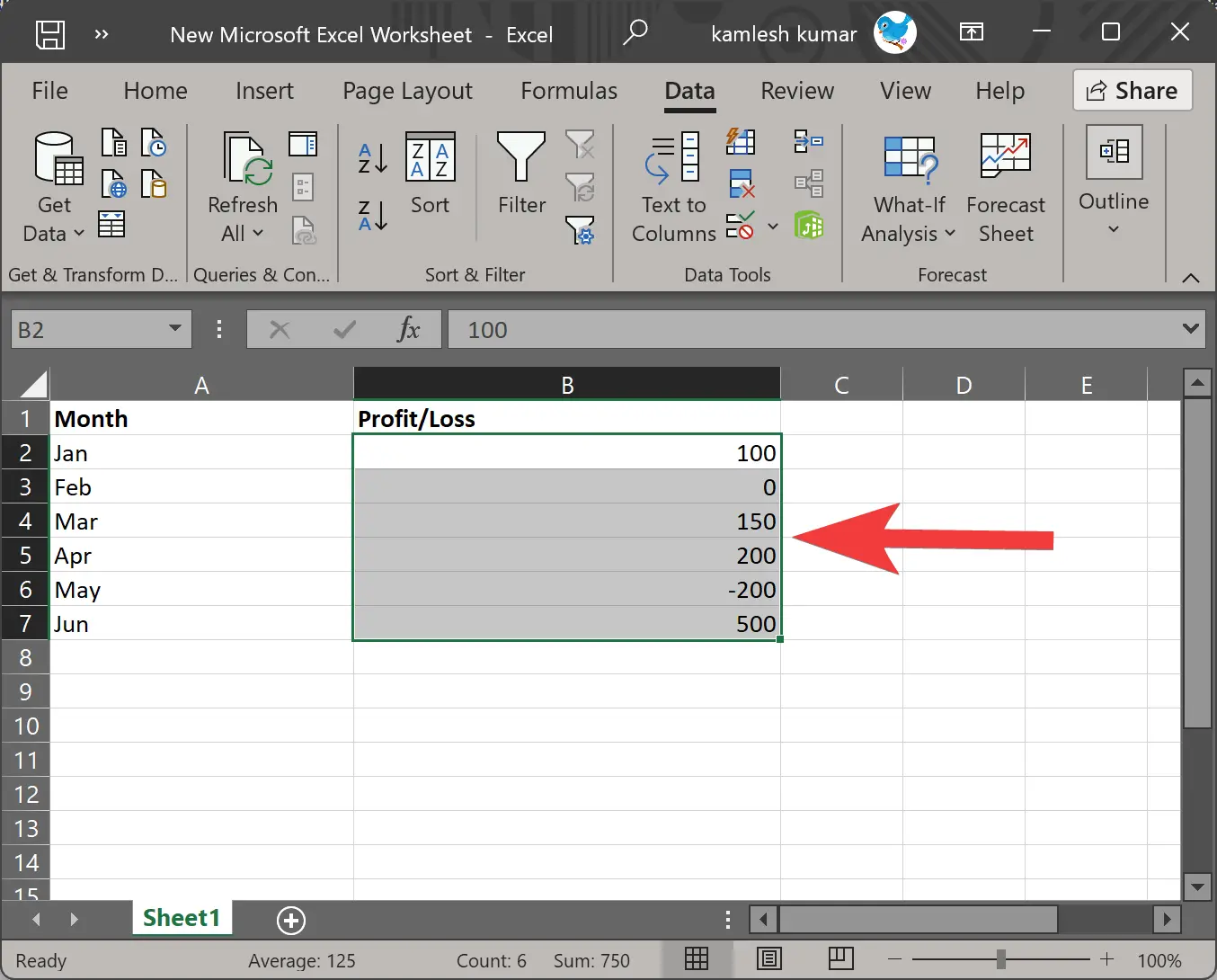
Step 1. Open your existing Microsoft Excel Worksheet or create a new one and fill in the data on that.
Step 2. Now, select the cells you want to change the format.
Step 3. Select the Home tab.
Step 4. In the “Number” section, click the small down arrow icon beside the Accounting Number Format icon.
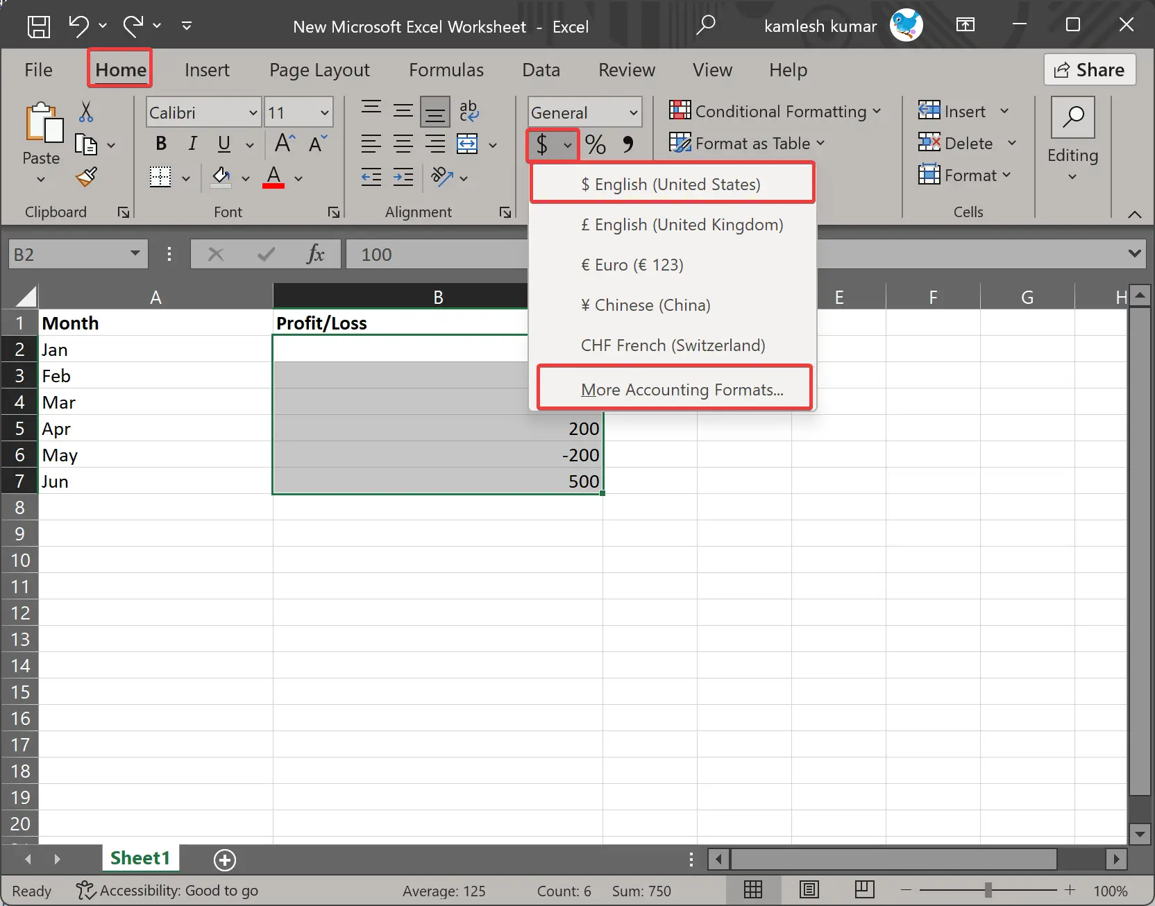
Step 5. Finally, select a currency type in the drop-down list.
If your country’s currency is not listed here, click on the More Accounting Formats option in the Accounting Number Format drop-down list and select your desired currency.
As an example, we have selected “$ English (United States),” and below is a screenshot of what our sheet looks like.
How to Use the Accounting Number Format through the Format Cells Dialog Box?
To use the Accounting Number Format through the Format Cells Dialog Box, follow these steps:-
Step 1. Open your existing Microsoft Excel Worksheet or create a new one and fill in the data on that.
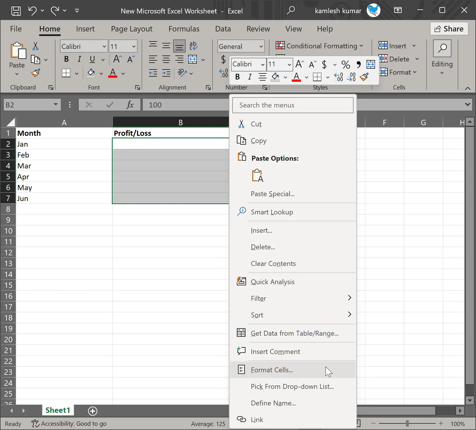
Step 2. Now, select the cells you want to change the format.
Step 3. Right-click on the chosen cells and select Format Cells in the pop-up menu. Alternatively, press Ctrl + 1 on your keyboard to open the Format Cells dialog box.
Step 4. In the Format Cells dialog, switch to the Number tab and then select Accounting in the left sidebar.
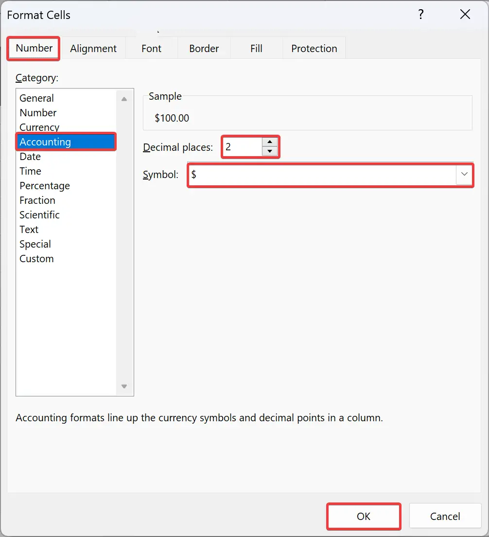
Step 5. The “Decimal places” box lets you select the number of decimals to display. Excel applies two decimals by default.
Step 6. Select your desired symbol to display in selected cells in the Symbol box.
Step 7. Click OK.
Now selected cells will display their values as accounting numbers.
Conclusion
In conclusion, Microsoft Excel is a powerful spreadsheet application that is widely used across various industries, with a special place in the business and accounting fields. The Accounting Number Format is a built-in feature in Excel that makes it easy for accountants to work with financial data. It allows for consistent formatting of financial values and has unique features, such as displaying zero values as a dash and negative values in parentheses. There are two ways to apply the Accounting Number Format in Excel: through the Accounting Number Format icon or the Format Cells Dialog Box. By following the steps outlined in this article, users can easily apply the Accounting Number Format in their Excel workbooks and make their financial data more readable and understandable.