Microsoft Excel is a powerful spreadsheet tool used by millions of people for data analysis, reporting, and various other tasks. Among its many functions, the TRANSPOSE function is a handy feature that allows you to change the orientation of your data, making it easier to work with.
In this gearupwindows article, we’ll explore what the TRANSPOSE function is, how to use it, and practical examples of when it can be beneficial.
What is the TRANSPOSE Function?
The TRANSPOSE function in Excel is designed to convert data from a vertical format to a horizontal one or vice versa. This can be especially useful when you need to reorganize data quickly, for instance, switching rows to columns or vice versa. This function simplifies the process, saving you time and effort.
How to Use the TRANSPOSE Function?
Using the TRANSPOSE function is straightforward. Here’s a step-by-step guide:-
Step 1. Launch Microsoft Excel and open a new or existing worksheet where you want to apply the TRANSPOSE function.
Step 2. Identify the range where you want to place the transposed data. This range should have enough empty cells to accommodate the transposed information.
Step 3. In the first cell of your destination range, type `=TRANSPOSE(.`
Step 4. Click and drag to select the range of data you want to transpose. This source range can be in the same or a different worksheet.
Step 5. After selecting the source range, close the function by typing a closing parenthesis `).` The formula in the destination cell should look like `=TRANSPOSE(SourceRange).`
Step 6. Instead of pressing just Enter, use Ctrl + Shift + Enter (known as an array formula) to confirm the formula. You will see the data transposed in your destination range.
– Alternatively, if you are using Excel 365 or Excel 2019, you can simply press Enter, and Excel will automatically apply the function as an array formula.
That’s it! You’ve successfully used the TRANSPOSE function to change the orientation of your data.
Practical Examples of TRANSPOSE function
Let’s look at a couple of practical examples of how the TRANSPOSE function can be useful:-
Example 1: Switching Rows to Columns
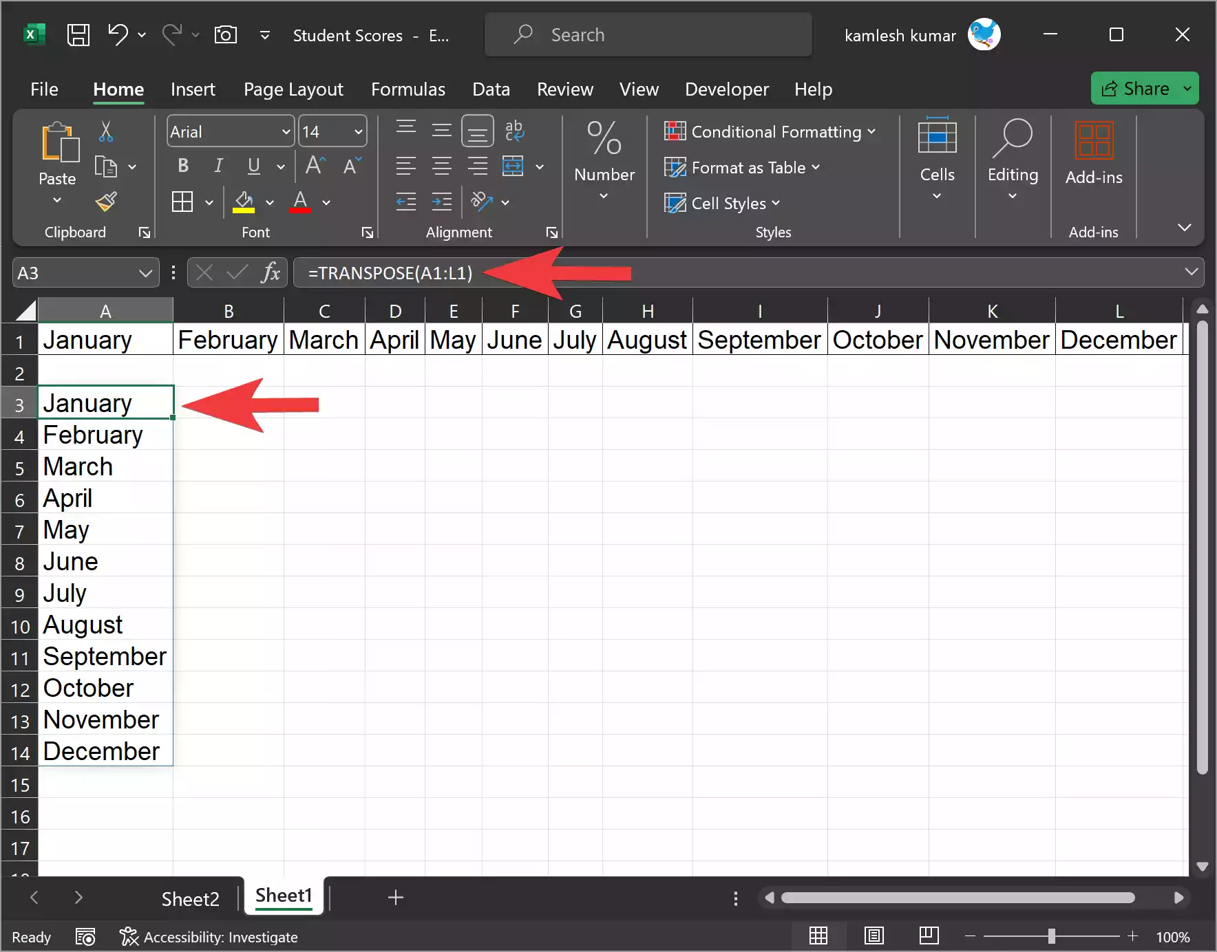
Suppose you have data where each row represents a different month, and you want to change it to a column format to create a summary. Here’s how you can do it with the TRANSPOSE function:-
Step 1. Select an empty range in your worksheet where you want the transposed data.
Step 2. Use the TRANSPOSE function with the source range containing your monthly data.
=TRANSPOSE(A1:L1)
Step 3. Press Ctrl + Shift + Enter (or Enter in newer Excel versions).

This will switch your data from a row format to a column format, making it easier to analyze and create charts.
Example 2: Combining Data from Multiple Worksheets
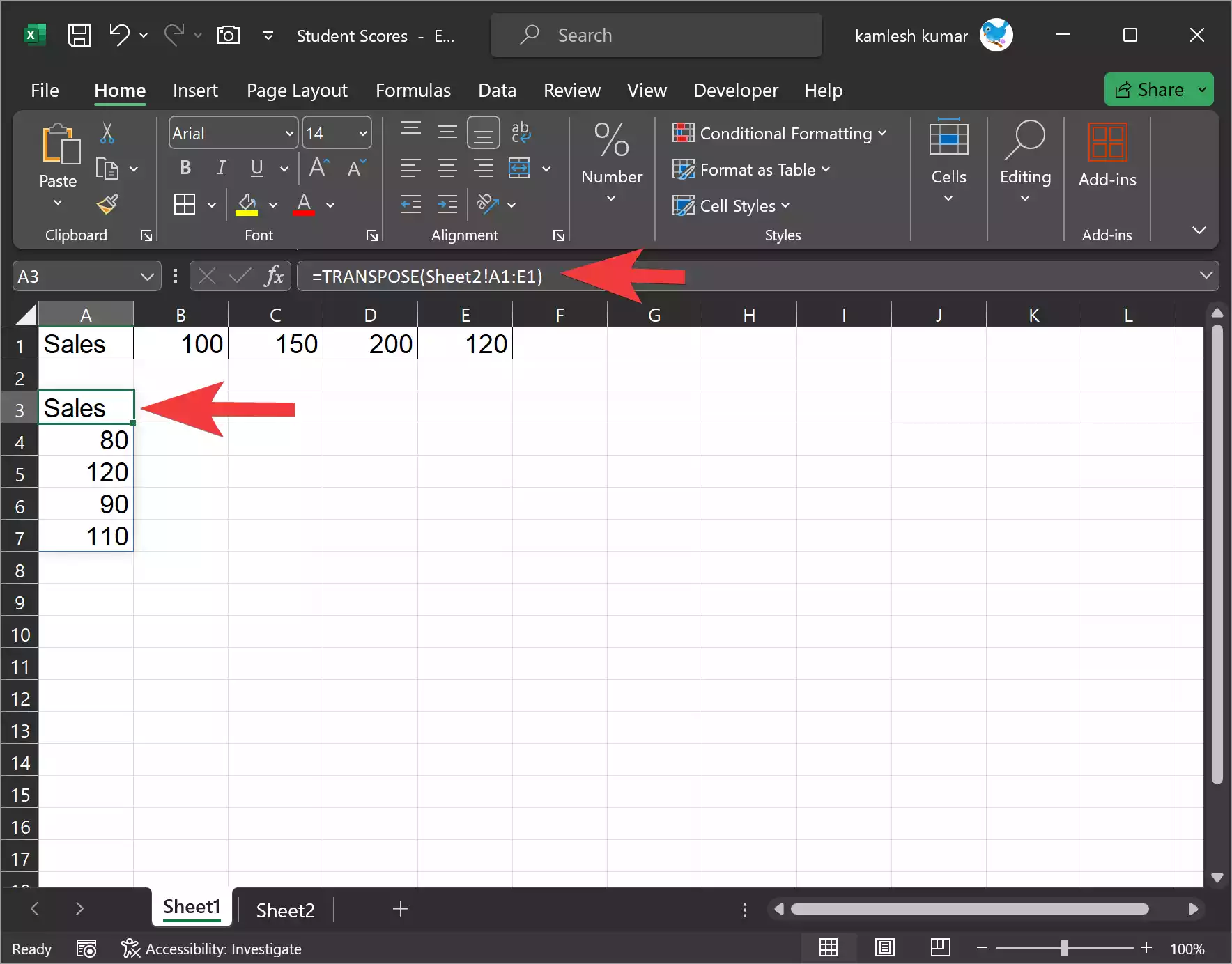
Suppose you have data in different worksheets representing different regions, and you want to combine this data into a single worksheet. You can use the TRANSPOSE function to accomplish this:
Step 1. In your destination worksheet, select an empty range where you want the combined data.
Step 2. Use the TRANSPOSE function with the source range in another worksheet.
=TRANSPOSE('Sheet2'!A1:E1)
Step 3. Press Ctrl + Shift + Enter (or Enter in newer Excel versions).

Repeat this process for each worksheet, and you’ll end up with a consolidated dataset in your destination worksheet.
Things to Consider
While the TRANSPOSE function is a powerful tool, there are some limitations and considerations to keep in mind:-
Step 1. The destination range must have enough space to accommodate the transposed data. If it’s too small, you’ll get a “Spill” error.
Step 2. If you’re using a version of Excel that supports dynamic arrays (Excel 365 or Excel 2019), you don’t need to use Ctrl + Shift + Enter. Excel will handle it automatically.
Step 3. The TRANSPOSE function only changes the data’s orientation. It won’t transpose any formatting, such as fonts or cell colors.
Step 4. When referencing data in other worksheets, make sure to enclose the sheet name in single quotes, like `‘Sheet2’!A1:A5.`
In Conclusion
The TRANSPOSE function in Excel is a handy tool for quickly changing the orientation of your data, making it easier to work with and analyze. Whether you need to switch rows to columns, combine data from multiple worksheets, or reorganize data for better readability, the TRANSPOSE function can save you time and effort in Excel. Experiment with it in different scenarios to discover its full potential in your data manipulation tasks.