Microsoft Excel is a versatile and powerful tool for managing and analyzing data. Among its many functions, the ability to sum a column or a range of cells is a fundamental and often-used feature. Whether you’re working with financial data, inventory lists, or any other type of data that requires adding up numbers, mastering the art of summing a column in Excel can significantly enhance your productivity and accuracy.
In this gearupwindows article, we’ll guide you through various methods to sum a column in Microsoft Excel, from the most basic to more advanced techniques.
How to Sum a Column in Microsoft Excel?
Method 1: The AutoSum Function
The simplest way to sum a column in Excel is by using the AutoSum function. Follow these steps:-
Step 1. Select the cell where you want the sum to appear (usually directly below the column you want to sum).

Step 2. Click on the “AutoSum” button located on the “Home” tab in the “Editing” group. It looks like a sigma (∑) symbol.

Step 3. Excel will automatically try to guess the range you want to sum. If it selects the correct range, press “Enter,” and the sum will appear in the selected cell.

Method 2: Manual Sum with the SUM Function
If the AutoSum function doesn’t work or if you want more control, you can use the SUM function. Here’s how:-
Step 1. Select the cell where you want the sum to appear.
Step 2. Type “=SUM(” in the formula bar.

Step 3. Click and drag to select the range of cells you want to sum.
Step 4. Close the formula by typing “)” and press “Enter.”
The sum of the selected cells will appear in the target cell.
Method 3: The Quick Analysis Tool
Excel offers a Quick Analysis tool that can speed up the process of summing a column. Here is how to use the Quick Analysis tool:-
Step 1. Select the column you want to sum.
Step 2. In the bottom-right corner of the selected range, a small icon (a square with a lightning bolt) will appear. Click on it.
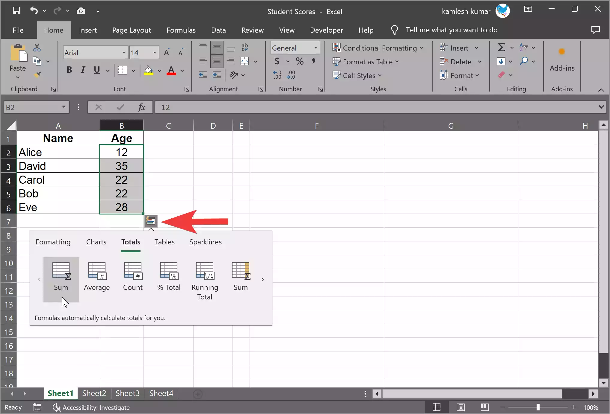
Step 3. A menu with various options will appear, including “Sum” under “Totals.” Click on “Sum.”
Excel will instantly calculate and display the sum at the bottom of the selected column.
Method 4: The SUBTOTAL Function
The SUBTOTAL function is a versatile tool for summing a column, especially when working with filtered data.
Step 1. Select the cell where you want the sum to appear.
Step 2. Type “=SUBTOTAL(109,” to begin the function. The “109” tells Excel to calculate the sum.
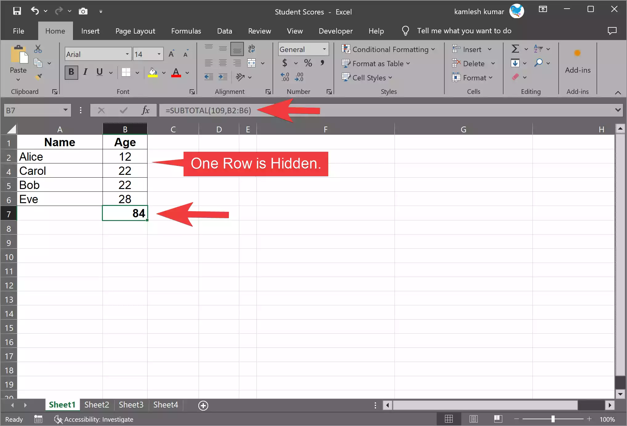
Step 3. Select the range you want to sum, even if it’s filtered.
Step 4. Close the formula by typing “)” and press “Enter.”
The SUBTOTAL function will calculate the sum of the selected range, considering any applied filters or hidden rows.
Method 5: Summing with PivotTables
For more advanced data analysis, PivotTables are a powerful tool. They can sum and analyze data in various ways. Here’s a simplified overview:-
Step 1. Select the range of data you want to summarize.
Step 2. Go to the “Insert” tab and select “PivotTable.”

Step 3. In the pop-up window, select “New Worksheet” or Existing Worksheet” and then select a cell to display the result.
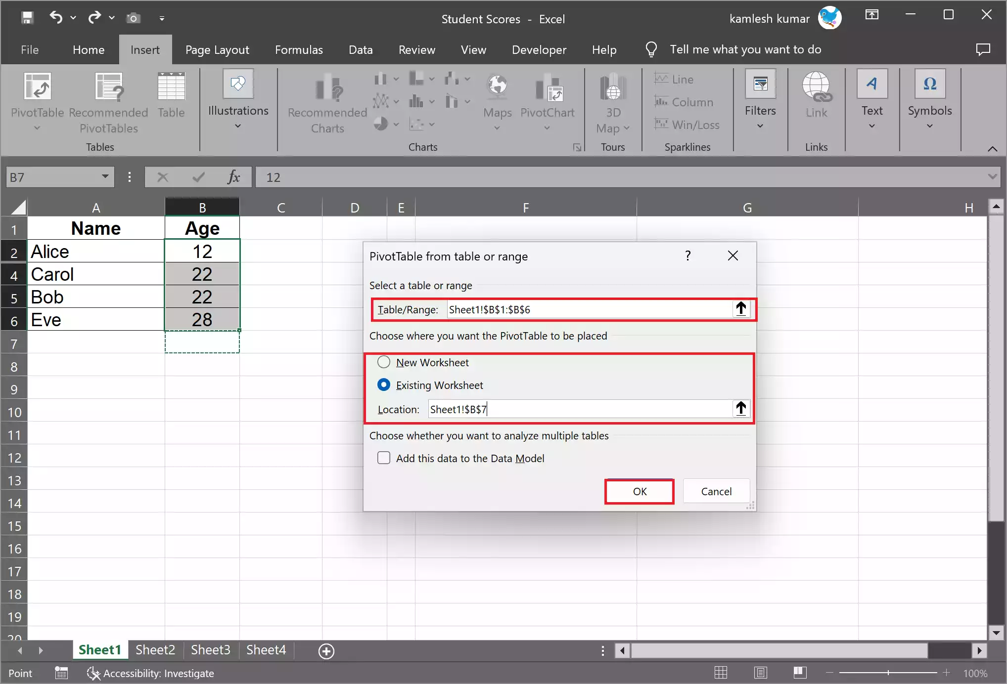
Step 4. When you’re done, click OK.
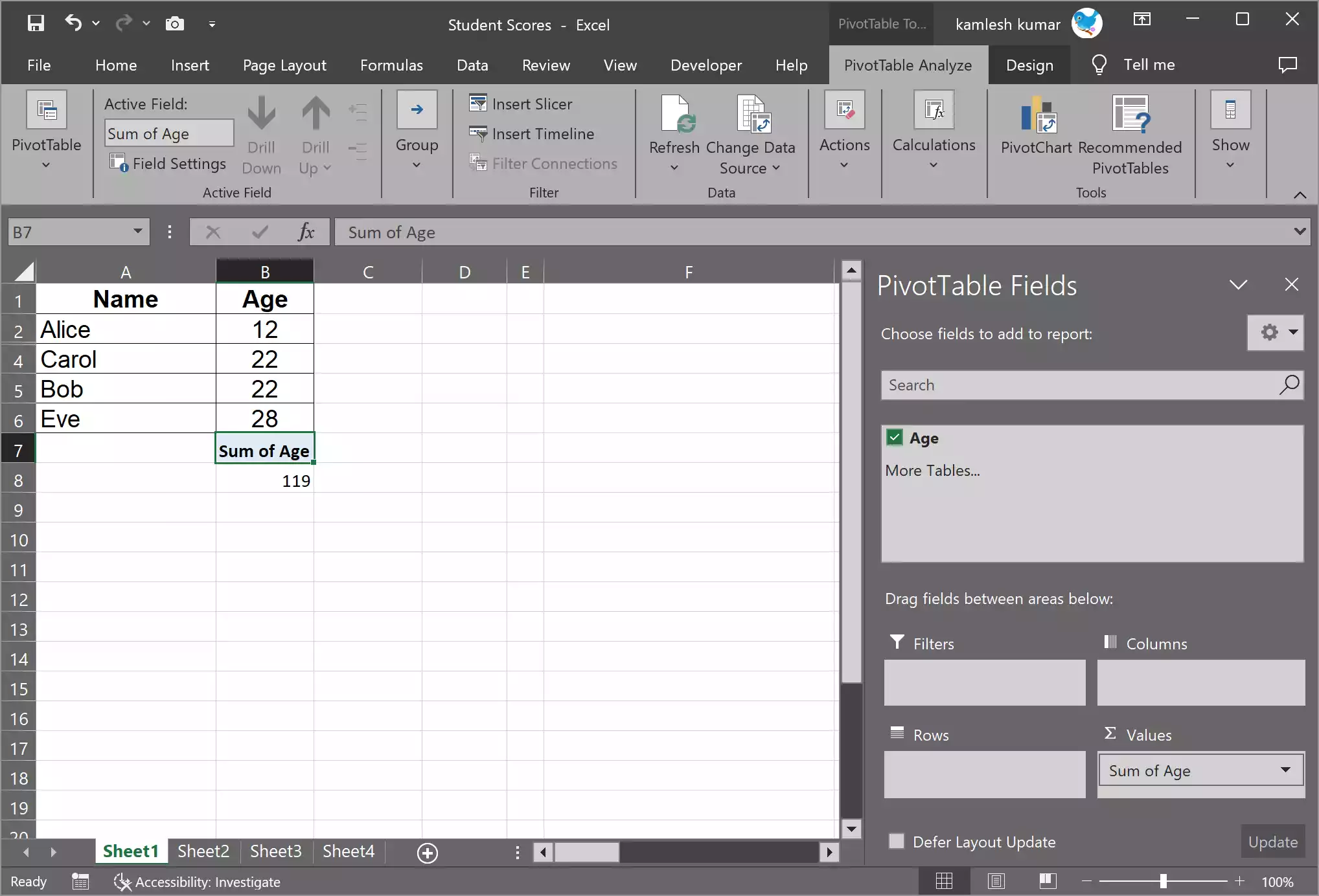
Step 5. In the PivotTable field list, drag and drop your column to the “Values” area.

Step 6. The PivotTable will automatically sum the values in your column and display the result.
Conclusion
Summing a column in Microsoft Excel is a fundamental skill that can significantly improve your data management and analysis capabilities. Whether you prefer the simplicity of AutoSum or the advanced features of PivotTables, Excel provides multiple methods to help you accomplish this task efficiently. By mastering these techniques, you can become more proficient in handling and extracting meaningful insights from your data, saving time and enhancing the accuracy of your work.
