Excel is a powerful tool for handling and analyzing data, and it offers a wide range of functions to help you manipulate and format your data efficiently. One such function that can be incredibly useful in Excel is the CONCATENATE function. In this gearupwindows article, we will explore how to use the CONCATENATE function to combine text and data from different cells into a single cell, making your data more organized and easier to work with.
What is CONCATENATE?
The CONCATENATE function in Excel is used to join or combine text from multiple cells into a single cell. This function can be particularly handy when you have data spread across different columns or rows and need to create a unified string of text for a specific purpose, such as creating mailing addresses, report headers, or custom labels.
The Syntax of CONCATENATE
The CONCATENATE function has a simple syntax. It takes multiple arguments, each representing the text or cell references you want to combine. Here’s the basic syntax:-
=CONCATENATE(text1, [text2], ...)
– `text1` (required): The first text or cell reference to combine.
– `text2`, `text3`, … (optional): Additional text or cell references to combine.
You can include up to 30 arguments in a single CONCATENATE function, allowing you to concatenate a substantial amount of data as needed.
How to Use the CONCATENATE Function in Excel?
Let’s walk through a step-by-step guide on how to use the CONCATENATE function:-
Step 1. Open Excel and select the cell where you want to display the concatenated text.
Step 2. Type the CONCATENATE function in the selected cell.
For example, if you want to combine the first name and last name from cells A2 and B2, your formula would look like this:-
=CONCATENATE(A2, " ", B2)
In this formula, we used the cell references A2 and B2, separated by a space enclosed in double quotation marks, to create a space between the first name and last name.
Step 3. Press Enter, and the result will be the concatenated text in the selected cell.
Step 4. Drag the fill handle to apply the formula to multiple rows or columns.
If you need to concatenate data for multiple rows or columns, you can drag the fill handle (a small square at the bottom-right corner of the cell) to copy the formula to adjacent cells. Excel will automatically adjust the cell references in the formula to match the new location.
Let’s walk through using the CONCATENATE function in Excel with examples and data.
Example 1: Combining First Name and Last Name
Suppose you have an Excel spreadsheet with a list of first names in column A and last names in column B. You want to create a single column with the full names. Here’s how you can do it:-
Step 1. Open Excel and select the cell where you want to display the concatenated names. In this example, let’s select cell C2.
Step 2. Type the CONCATENATE function in cell C2:-
=CONCATENATE(A2, " ", B2)
This formula will combine the first name from cell A2, add a space, and then concatenate it with the last name from cell B2.
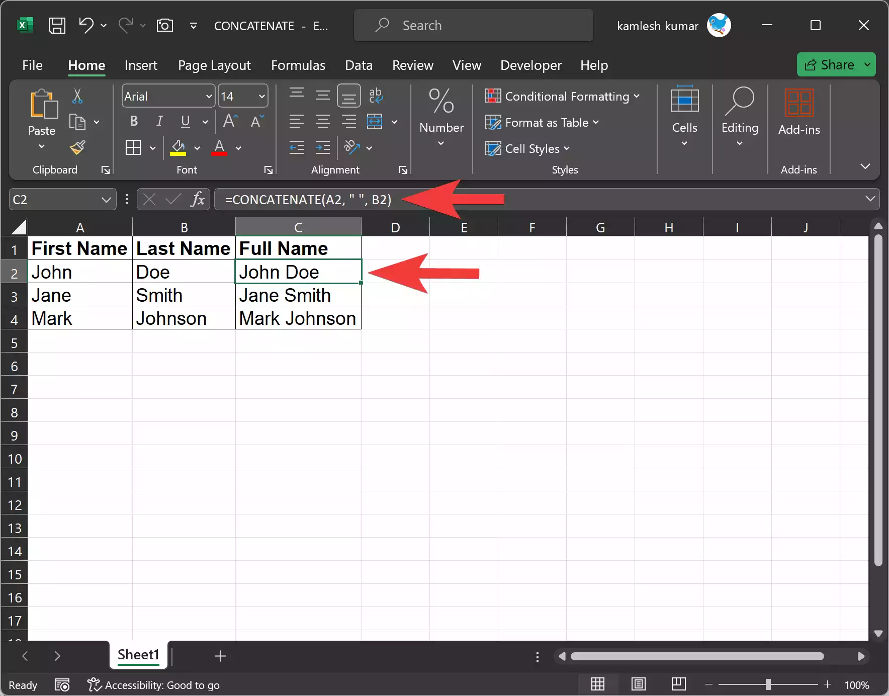
Step 3. Press Enter.
Cell C2 now displays the full name, which is the result of concatenating the first name and last name.
Step 4. Drag the fill handle (the small square at the bottom-right corner of cell C2) down to apply the formula to multiple rows.
Excel will automatically adjust the cell references as you drag the fill handle, creating concatenated full names for each row.
Example 2: Combining Text and Numbers
Let’s say you have a list of product names in column A and their corresponding prices in column B. You want to create a description that includes the product name and its price. Here’s how you can do it:-
Step 1. Open Excel and select the cell where you want to display the concatenated descriptions. Let’s choose cell C2 again.
Step 2. Type the CONCATENATE function in cell C2:-
=CONCATENATE("Product: ", A2, " - Price: $", B2)
In this formula, we use text within double quotation marks to add labels (“Product: ” and ” – Price: $”) as delimiters between the product name (from cell A2) and the price (from cell B2).
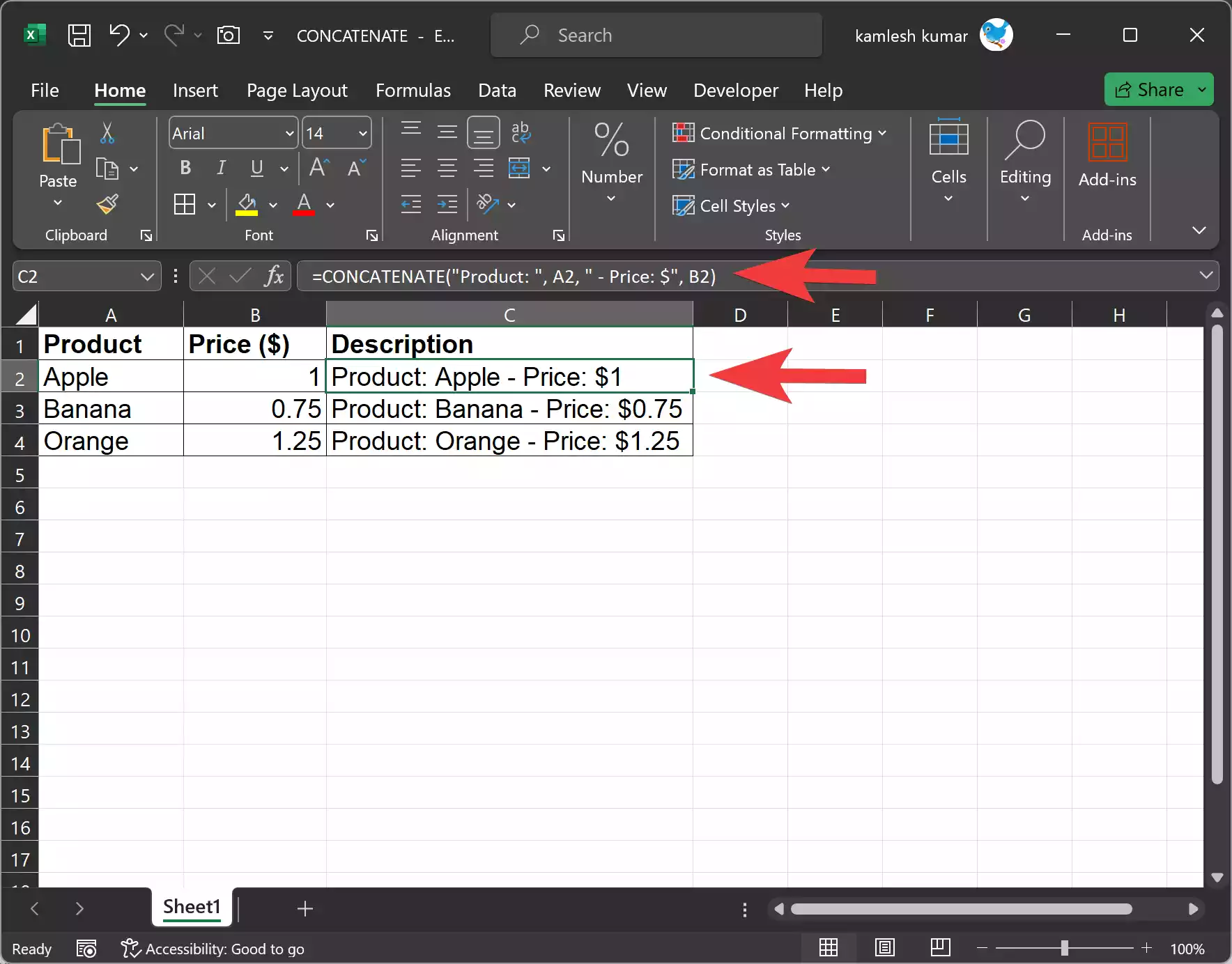
Step 3. Press Enter.
Cell C2 now displays the product description, which includes the product name and its price.
Step 4. Drag the fill handle down to apply the formula to other rows.
Excel will adjust the cell references to create unique descriptions for each product.
These examples demonstrate how to use the CONCATENATE function in Excel to combine text and data from different cells, making your data more organized and suitable for various purposes. Whether you’re dealing with names, descriptions, or addresses, CONCATENATE simplifies the process of consolidating data in Excel.
Additional Tips and Tricks
1. Adding Delimiters: You can use text within double quotation marks as delimiters to separate the concatenated values. In our example, we used a space as a delimiter between the first name and last name.
2. Mixing Text and Numbers: You can combine text and numeric values using the CONCATENATE function. Excel will treat numbers as text when concatenating.
3. Handling Empty Cells: If one of the cells you’re trying to concatenate is empty, the CONCATENATE function will still work, but it will include the empty cell as an empty space in the result.
4. Ampersand Operator: In addition to the CONCATENATE function, you can also use the ampersand (`&`) operator to achieve the same result. For example, `=A2&” “&B2` would concatenate the first name and last name just like our earlier CONCATENATE example.
Conclusion
The CONCATENATE function in Excel is a valuable tool for merging text and data from different cells into a single, more organized format. Whether you’re creating reports, labels, or custom data strings, understanding how to use CONCATENATE can save you time and effort by simplifying the data consolidation process.