Microsoft Excel is a powerful spreadsheet tool that allows you to manage, analyze, and visualize data effectively. One of its standout features is Conditional Formatting, which enables you to apply formatting rules to cells or ranges based on specified conditions. This capability is invaluable for highlighting key data points, trends, and anomalies in your datasets, making it easier to derive insights and make informed decisions. In this article, we’ll explore the ins and outs of Conditional Formatting in Excel and demonstrate how it can enhance your data analysis.
What is Conditional Formatting?
Conditional Formatting is a feature in Excel that allows you to format cells based on certain criteria or conditions. Instead of manually formatting each cell individually, you can set up rules that automatically format cells that meet specific conditions. This not only saves time but also makes your data visually informative.
How to Apply Conditional Formatting?
Let’s dive into the steps to apply Conditional Formatting in Excel:-
Step 1. First, select the range of cells to which you want to apply Conditional Formatting to. You can select a single cell, a row, a column, or a larger range, depending on your needs.
Step 2. Go to the “Home” tab on the Excel ribbon. In the “Styles” group, you’ll find the “Conditional Formatting” button. Click on it to access various Conditional Formatting options.
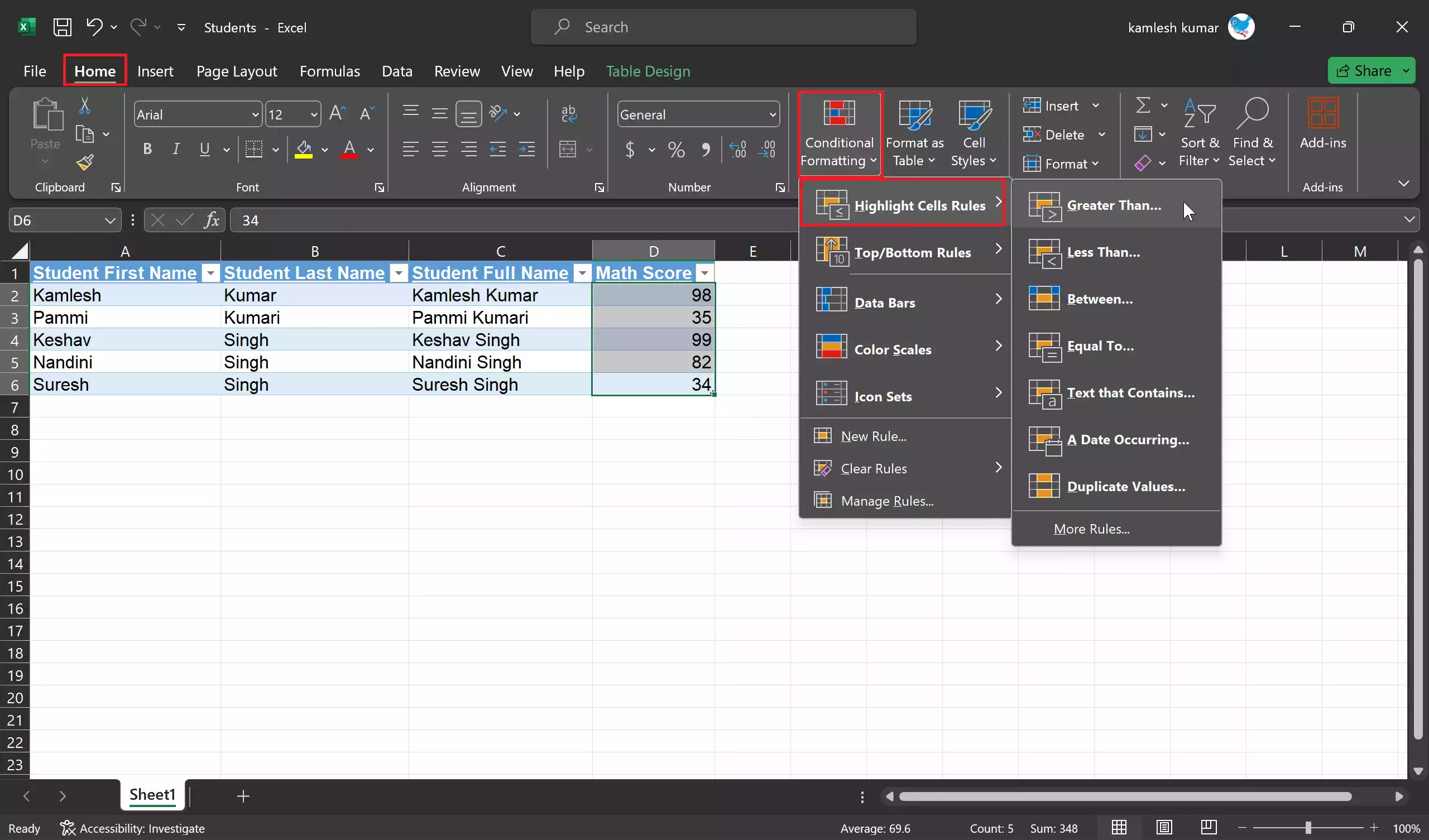
Step 3. Excel offers several built-in rules for Conditional Formatting, such as highlighting cells that contain specific text, values greater or less than a certain threshold, duplicate values, and more. Select the rule that suits your data analysis goals.
Step 4. After selecting a rule, you’ll need to define the conditions and formatting options. For example, if you choose the rule “Highlight Cells Rules” > “Greater Than,” you’ll need to specify the value and choose a format style like bold text or a specific fill color.
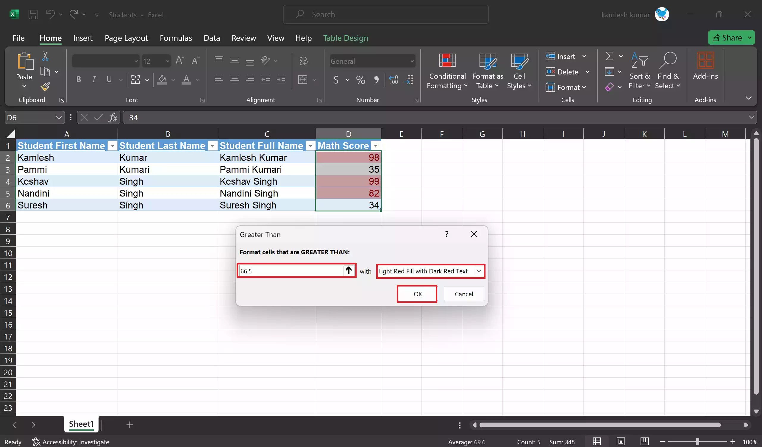
Step 5. Excel provides a preview of how the formatting will look on your selected data. Review it to ensure it meets your requirements, and then click “OK” to apply the Conditional Formatting.
Practical Applications of Conditional Formatting
Now, let’s explore some practical ways in which Conditional Formatting can be used to gain better insights from your data:-
- Identifying Trends: Conditional Formatting can help you quickly spot trends in your data. For example, you can use color scales to visualize data gradients, making it easier to identify high and low values. This is especially useful for heatmaps and data comparisons.
- Data Validation: Ensure data accuracy and consistency by using Conditional Formatting to highlight cells that contain errors or don’t meet certain criteria. For instance, you can highlight all negative numbers in red to draw attention to potential issues.
- Prioritizing Data: Highlight the most important information in your dataset by applying Conditional Formatting to cells that meet specific criteria. For instance, you can make overdue tasks in a project management spreadsheet stand out by applying a bold red font to their due dates.
- Spotting Anomalies: Identify outliers or unusual data points by setting up Conditional Formatting rules that highlight values outside a specified range. This is particularly useful for quality control and anomaly detection.
- Creating Gantt Charts: Conditional Formatting can be used to create simple Gantt charts by applying different fill colors to date ranges. This helps visualize project timelines and task dependencies.
Tips for Effective Conditional Formatting
To make the most of Conditional Formatting in Excel, consider the following tips:-
- Use Color Wisely: While color can be a powerful tool, excessive use can make your spreadsheet cluttered and confusing. Stick to a limited color palette and be consistent.
- Clear Formatting: Excel allows you to clear Conditional Formatting from selected cells or ranges if you want to start fresh or make changes.
- Order of Rules: Rules are applied in the order they appear in the Conditional Formatting Rules Manager. Pay attention to rule precedence when you have multiple rules affecting the same cells.
- Cell References: When setting up Conditional Formatting rules, use absolute or mixed cell references ($A$1) to ensure the rules work as expected when applied to other cells.
- Data Bars and Icon Sets: Explore advanced Conditional Formatting options like data bars and icon sets for more visual variations.
Conclusion
Conditional Formatting is a powerful feature in Excel that can help you make your data more visually appealing and informative. By highlighting data based on specific conditions, you can quickly identify patterns, trends, and outliers in your datasets. Whether you’re a business analyst, a project manager, or a student, mastering Conditional Formatting will undoubtedly enhance your data analysis skills and enable you to make better-informed decisions based on your data insights. So, start exploring this feature and unlock the full potential of your Excel spreadsheets.
Also Read: