Microsoft Excel is a powerful spreadsheet program that offers a wide range of functions to help users manipulate and analyze data. One of these functions is the CEILING function. The CEILING function allows you to round a number up to the nearest specified multiple, making it useful in various financial and mathematical calculations. In this gearupwindows article, we’ll explore what the CEILING function is, how to use it, and provide some practical examples.
Understanding the CEILING Function
The CEILING function is used to round a number up to the nearest multiple you specify. It is particularly useful when you need to ensure that a value is always rounded up to the nearest increment, such as when working with pricing, quantities, or other financial calculations. The syntax for the CEILING function is as follows:-
CEILING(number, significance)
– `number`: This is the value you want to round up to the nearest multiple.
– `significance`: This is the multiple to which you want to round the number.
How to Use CEILING Function in Microsoft Excel?
To use the CEILING function in Excel, follow these steps:-
Step 1. Launch Microsoft Excel and create a new worksheet or open an existing one where you want to perform the rounding.
Step 2. Click on the cell where you want the rounded value to appear.
Step 3. In the selected cell, type the following formula, replacing `number` and `significance` with your specific values:-
=CEILING(number, significance)
Step 4. After entering the formula, press the “Enter” key, and Excel will calculate the rounded value.
Practical Examples
Let’s go through a few practical examples to demonstrate how to use the CEILING function in Excel.
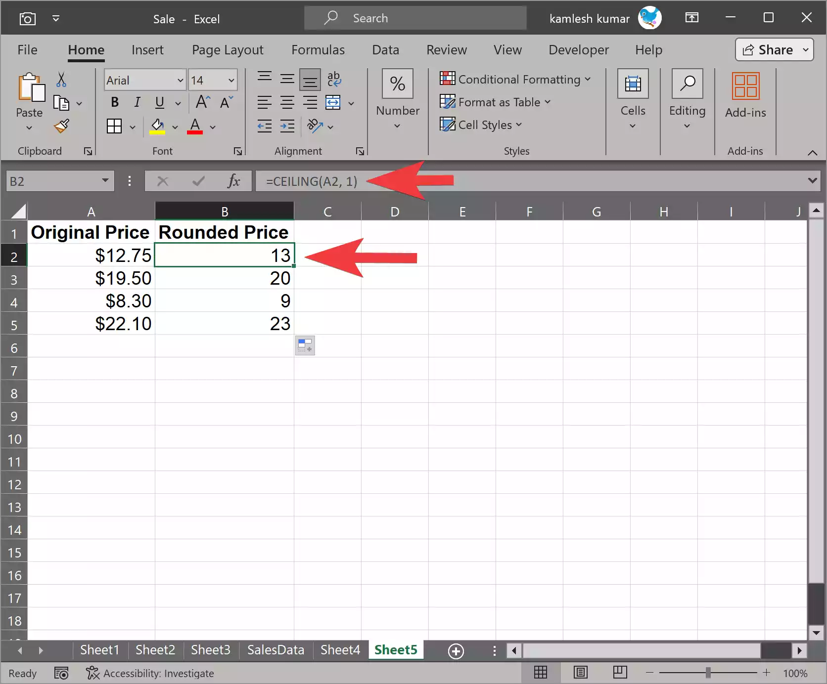
Example 1: Rounding Up Prices
Suppose you have a list of product prices, and you want to round them up to the nearest dollar. In this case, you can use the CEILING function. Assuming the original price is in cell A2, and you want the rounded price to appear in cell B2, you can enter the following formula in cell B2:
=CEILING(A2, 1)
This formula will round the price in A2 up to the nearest dollar.
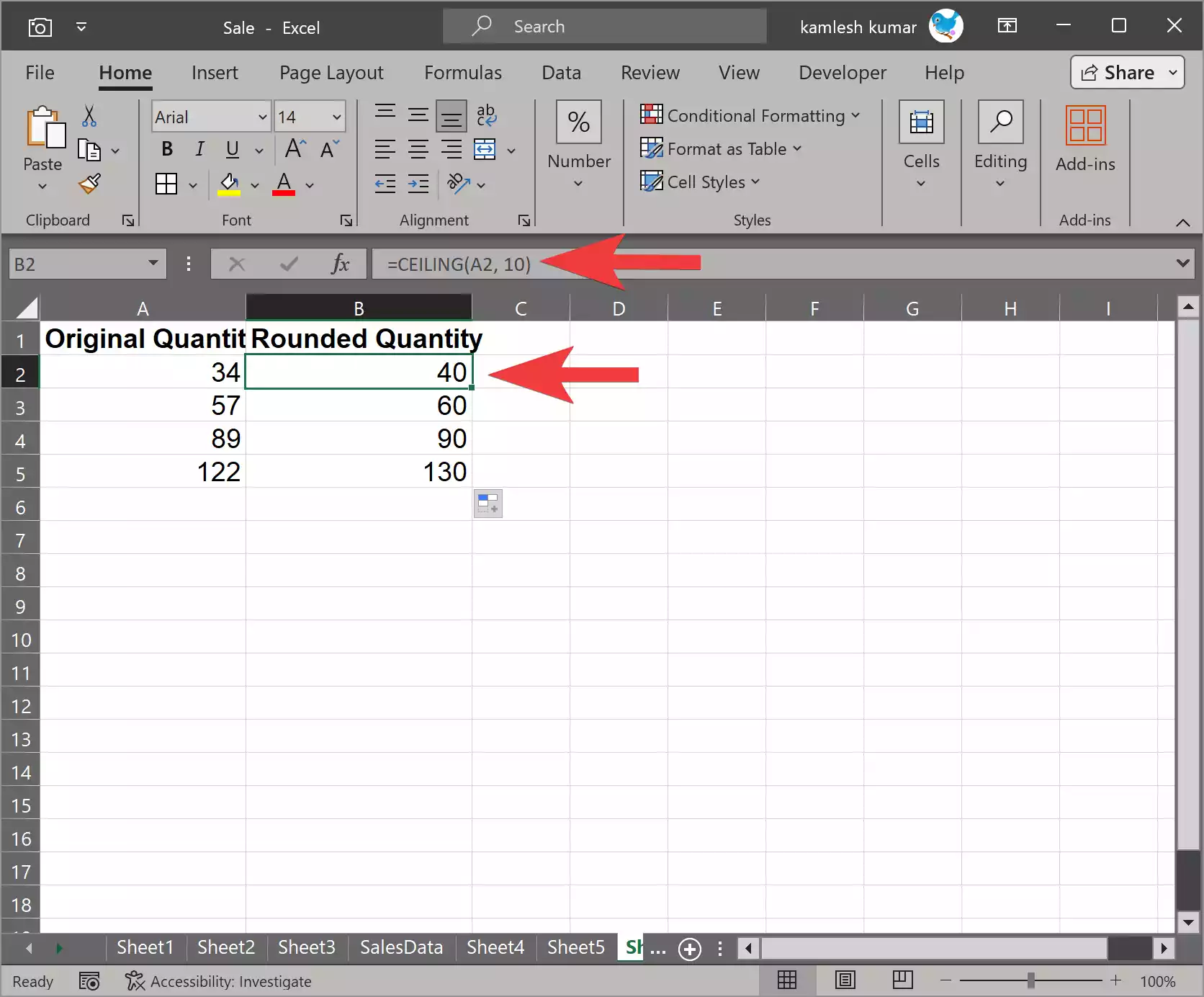
Example 2: Rounding Up Quantity
Let’s say you have a list of quantities, and you want to round them up to the nearest 10. If the original quantity is in cell A2, and you want the rounded quantity to appear in cell B2, you can use the CEILING function like this:-
=CEILING(A2, 10)
This formula will round the quantity in A2 up to the nearest multiple of 10.
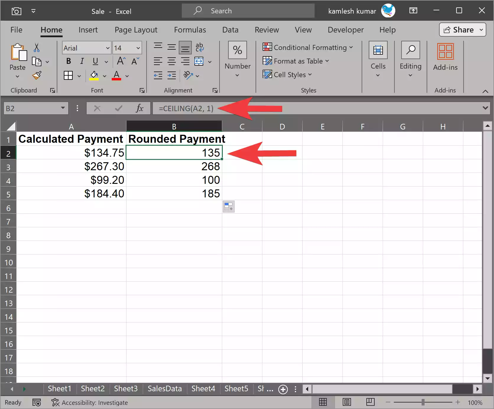
Example 3: Rounding Up for Loan Payments
Suppose you are calculating monthly loan payments and want to ensure that the payments are always rounded up to the nearest dollar. If the calculated payment is in cell A2, and you want the rounded payment to appear in cell B2, you can use the CEILING function as follows:-
=CEILING(A2, 1)
This formula will ensure that the monthly payment in B2 is always rounded up to the nearest dollar.
Conclusion
The CEILING function in Microsoft Excel is a valuable tool for rounding numbers up to specified multiples. It is particularly useful in financial and mathematical scenarios where precision and consistency in rounding are important. By following the steps outlined in this article and practicing with different examples, you can make the most of the CEILING function and improve the accuracy of your calculations in Excel.
Also Read: