
Microsoft Excel is a versatile spreadsheet application used for a wide range of tasks, from simple data entry to complex data analysis. One common task is counting the number of checkboxes in a worksheet, which can be particularly useful when you’re working with forms or to keep track of completed tasks in a to-do list. In this gearupwindows article, we’ll explore several methods to count checkboxes in Microsoft Excel.
How to Count Checkboxes in Microsoft Excel?
Method 1. Using COUNTIF Function
The COUNTIF function is a simple way to count the number of checkboxes in an Excel worksheet. Here’s how you can do it:-
Step 1. Select a cell where you want to display the count.
Step 2. Enter the following formula:-
=COUNTIF(range, TRUE)
Replace “range” with the actual range of cells that contain your checkbox results. This formula will count all the checkbox results with a checked (TRUE) state.
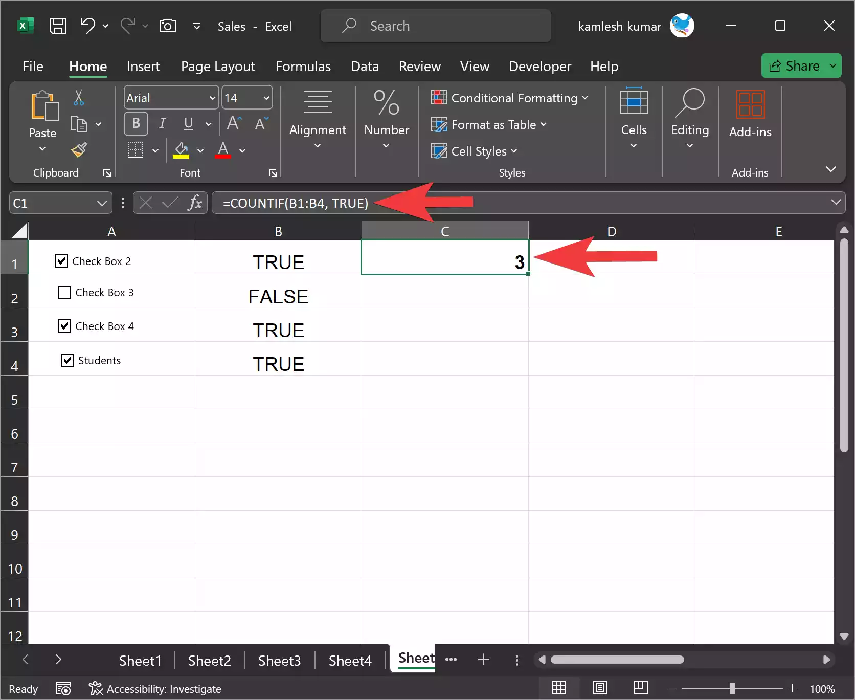
Step 3. Press Enter, and the cell will display the count of checkboxes in the specified range.
Note: If you want to count the unchecked boxes instead, simply replace True with False in the formula:-
=COUNTIF(range, FALSE)
Method 2: Using a Helper Column
If you prefer to use a non-formulaic solution, you can use a helper column to count the checkboxes. Here’s how:-
Step 1. Insert a new column adjacent to your checkboxes.
Step 2. In the first cell of the new column, enter the formula `=IF(B1=TRUE, 1, 0)`, assuming your checkboxes are in column B. Adjust the reference to your specific column as needed.

Step 3. Copy this formula down to cover all the checkboxes.
Step 4. In a separate cell, use the `SUM` function to add up the values in the helper column, which will give you the count of checked checkboxes. The formula in cell D1 can be:-
=SUM(C1:C5)
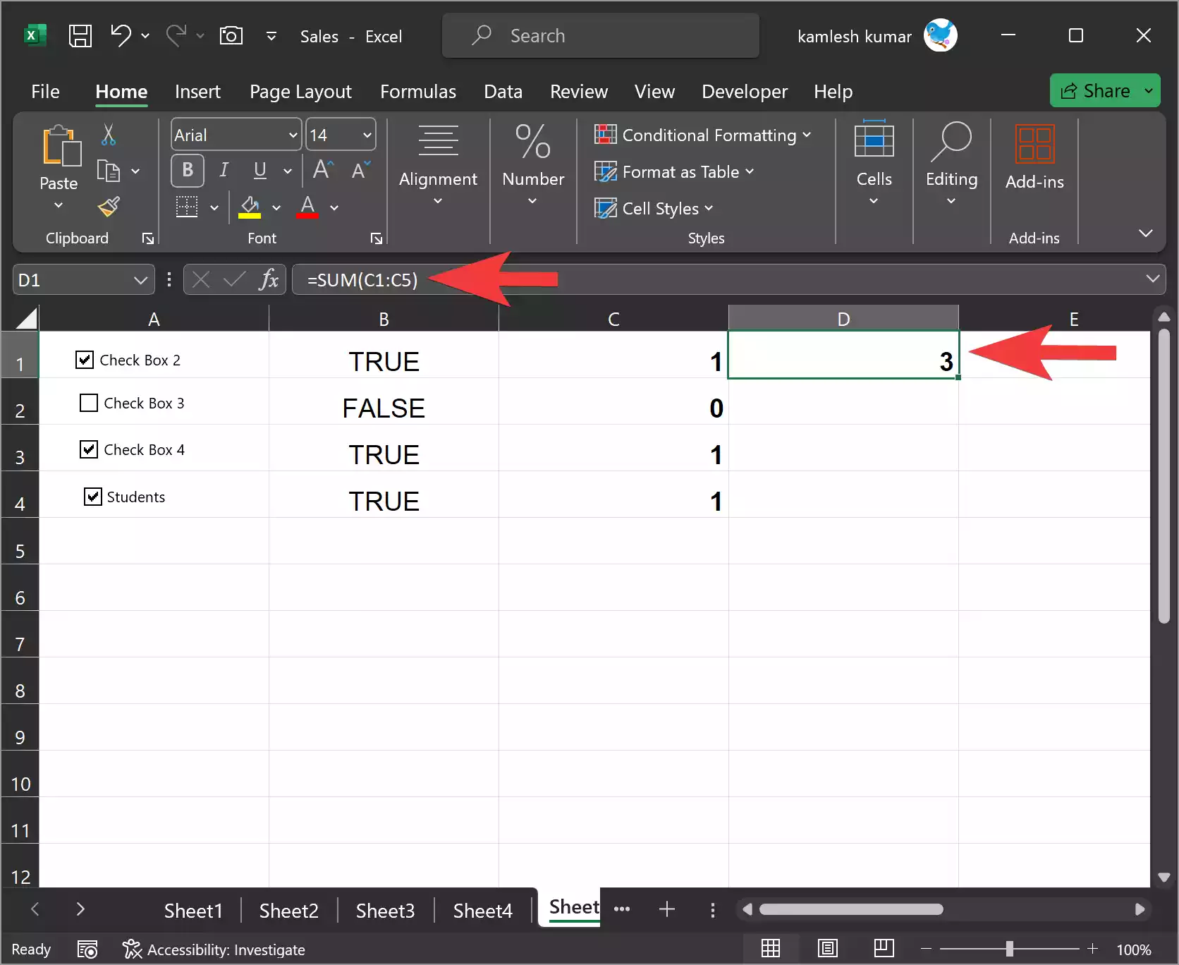
This method allows you to visually see which checkboxes are counted.
Method 3. Using Conditional Formatting
If you want a more visual approach, you can use conditional formatting to highlight the checked checkboxes and then count the highlighted cells. Here’s how:-
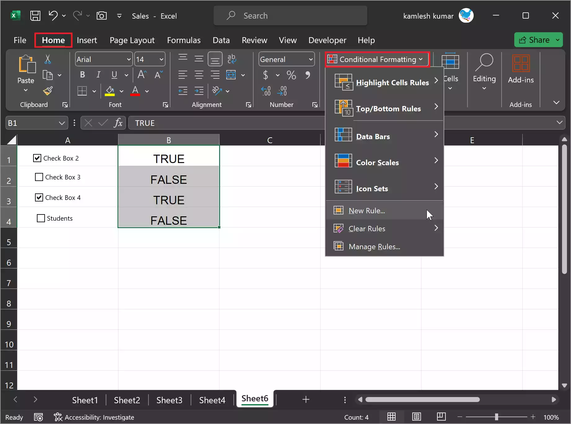
Step 1. Select the range of cells containing checkboxes.
Step 2. Go to the “Home” tab in the Excel ribbon.
Step 3. Click on “Conditional Formatting” and then choose “New Rule.”
Step 4. Select “Use a formula to determine which cells to format.”
Step 5. Enter the formula `=B1=TRUE` (assuming your checkboxes are in column B) and then click on the Format button to format style to highlight the checked checkboxes.

Step 6. In the “Format Cells” dialog box, choose a color of your choice in the “Fill” tab.

Step 7. Click OK.
Step 8. Click “OK” to apply the formatting.
After applying the conditional formatting, the checked checkboxes will be highlighted. You can now count the highlighted cells visually.
There are several methods to count checkboxes in Microsoft Excel. Depending on your preferences and the complexity of your spreadsheet, you can choose the method that suits your needs best. Whether you prefer using simple formulas, helper columns, or conditional formatting, Excel provides various options to count checkboxes efficiently.